Data Simulation

This section describes the steps to simulate occurrence data for fitting spatially explicit occupancy models in R-INLA.

Caution

Make sure you have that latest R and R-INLA versions installed:

R version 4.4.0 or above

R-INLA version INLA_24.06.04 or above. For latest testing version use:

install.packages("INLA",
        repos=c(getOption("repos"),
        INLA="https://inla.r-inla-download.org/R/testing"), dep=TRUE)

1 Set up

Code

# Load the libraries
library(INLA)
library(inlabru)
library(fmesher)
library(tidyverse)
library(spatstat)
library(sf)
library(terra)
library(ggplot2)
library(gt)
library(dplyr)
library(viridis)
library(viridisLite)
library(scico)
library(patchwork)

Define the spatial domain and the regular lattice by setting a \(300 \times 300\) study area divided into \(3\times3\) grid cells.

Code

# Define spatial domain
win <- owin(c(0,300), c(0,300))
npix <- 1000

Domain <- rast(nrows=npix, ncols=npix,
               xmax=win$xrange[2],xmin=win$xrange[1],
               ymax = win$yrange[2],ymin=win$yrange[1])

values(Domain) <- 1:ncell(Domain)
xy <- crds(Domain)

# Define regular grid
cell_size = 3
customGrid <- st_make_grid(Domain,cellsize = c(cell_size,cell_size)) %>% 
  st_cast("MULTIPOLYGON") %>%
  st_sf() %>%
  mutate(cellid = row_number())

# number of cells
ncells <- nrow(customGrid)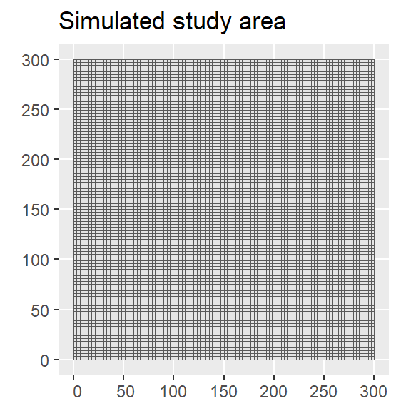

Figure 1: Custom 5\(^2\) units regular grid over a \(300^2\) area .

2 Simulate data for a simple spatial occupancy model

We simulate three different Gaussian Markov Random fields (GMRF) using the inla.qsample function.

Code

# Spatial boundary
boundary_sf = st_bbox(c(xmin = 0, xmax = 300, ymax = 0, ymin = 300)) %>%
  st_as_sfc()

# Create a fine mesh
mesh_sim = fm_mesh_2d(loc.domain = st_coordinates(boundary_sf)[,1:2],
                offset = c(-0.1, -.2),
                 max.edge = c(4, 50))
# Matern model
matern_sim <- inla.spde2.pcmatern(mesh_sim,
                                  prior.range = c(100, 0.5),
                                  prior.sigma = c(1, 0.5))


range_spde = 100
sigma_spde = 1

# Precision matrix
Q = inla.spde.precision(matern_sim, theta = c(log(range_spde),
                                              log(sigma_spde)))
# Simulate three spatial fields
seed = 12345
sim_field = inla.qsample(n = 3, Q = Q, seed = seed)

Create the projector matrix A_proj using the centroid of each grid cell as coordinates and compute the spatial random effect \(\omega(s)\), spatial environmental covariate \(x(s)\) and spatial detection covariate \(g_1(s)\) (Figure 2). (Note: Covariates \(x(s)\) and \(g_1(s)\) are assumed to be known and are stored as raster data).

Code

# Obtain the centroid of each cell
coord_grid  = st_coordinates(customGrid %>% st_centroid())
# A matrix
A_proj = inla.spde.make.A(mesh_sim, loc = coord_grid)

# Spatial components
omega_s = (A_proj %*% sim_field)[,1] # spatial random field
x_s = (A_proj %*% sim_field)[,2] # spatial environmental covariate
g_s = (A_proj %*% sim_field)[,3] # spatial detection covariate

# create rasters
x_rast = rast(data.frame(x = coord_grid[,1], y = coord_grid[,2],x_s))
g_rast = rast(data.frame(x = coord_grid[,1], y = coord_grid[,2],g_s))

# save raster data

writeRaster(x_rast,filename = paste('raster data','x_covariat.tif',sep='/'),
            overwrite=TRUE)
writeRaster(g_rast,filename = paste('raster data','g_covariat.tif',sep='/'),overwrite=TRUE)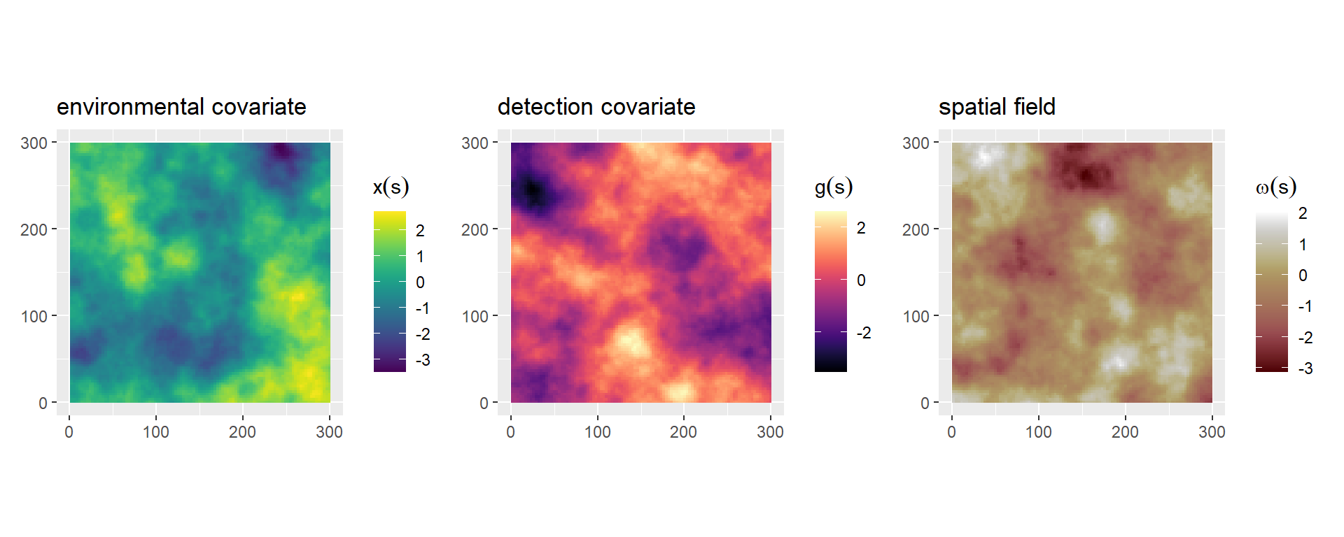

Figure 2: Simulated environmental and detection spatial covariates, and spatial occupancy random field.

Occurrence data is simulated from the following occupancy model:

\[\begin{align} \mbox{State process:}& \begin{cases} z_i \sim \mathrm{Bernoulli}(\psi_i) \nonumber \\\mathrm{logit}(\psi_i) = \beta_0 + \beta_1 \ x_i(s) + \omega_i(s) \\ \end{cases}\\ \mbox{ Observational process:}& \begin{cases} y_{ij} \sim \mathrm{Bernoulli}(z_i \times p_{ij}) \nonumber \\\mathrm{logit}(p_{ij}) = \alpha_0 + \alpha_1 \ g_{1i}(s) + \alpha_2 \ g_{2ij}\\ \end{cases} \end{align}\]

Here, \(g_{2}\) is a survey-level covariate that allows detection probabilities to vary between visits/surveys ( see Section 2.2 for simulation details).

2.1 State process model sub-component

Define model parameters \(\beta\) and compute the occupancy probabilities \(\psi\) and occupancy states \(z\) (Figure 3)

Code

# State process model coeficcients
beta <- c(NA,NA)
beta[1] <-  qlogis(0.3) # Base line occupancy probability
beta[2] <- 1.5  # environmental covariate effect

# Occupancy probabilities
psi <- inla.link.logit(beta[1] + beta[2]*x_s + omega_s, inverse = T)

# True occupancy state

set.seed(seed)
z <- rbinom(ncells, size = 1, prob = psi)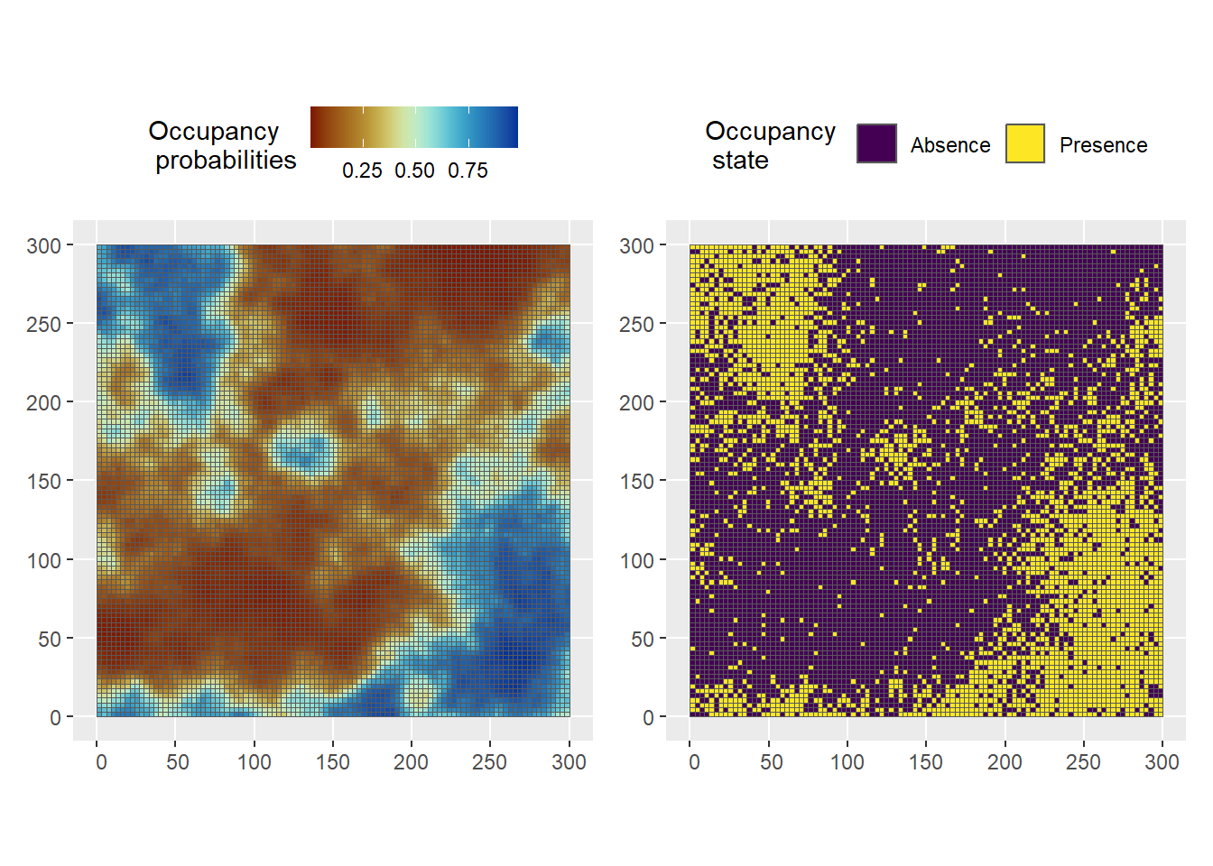

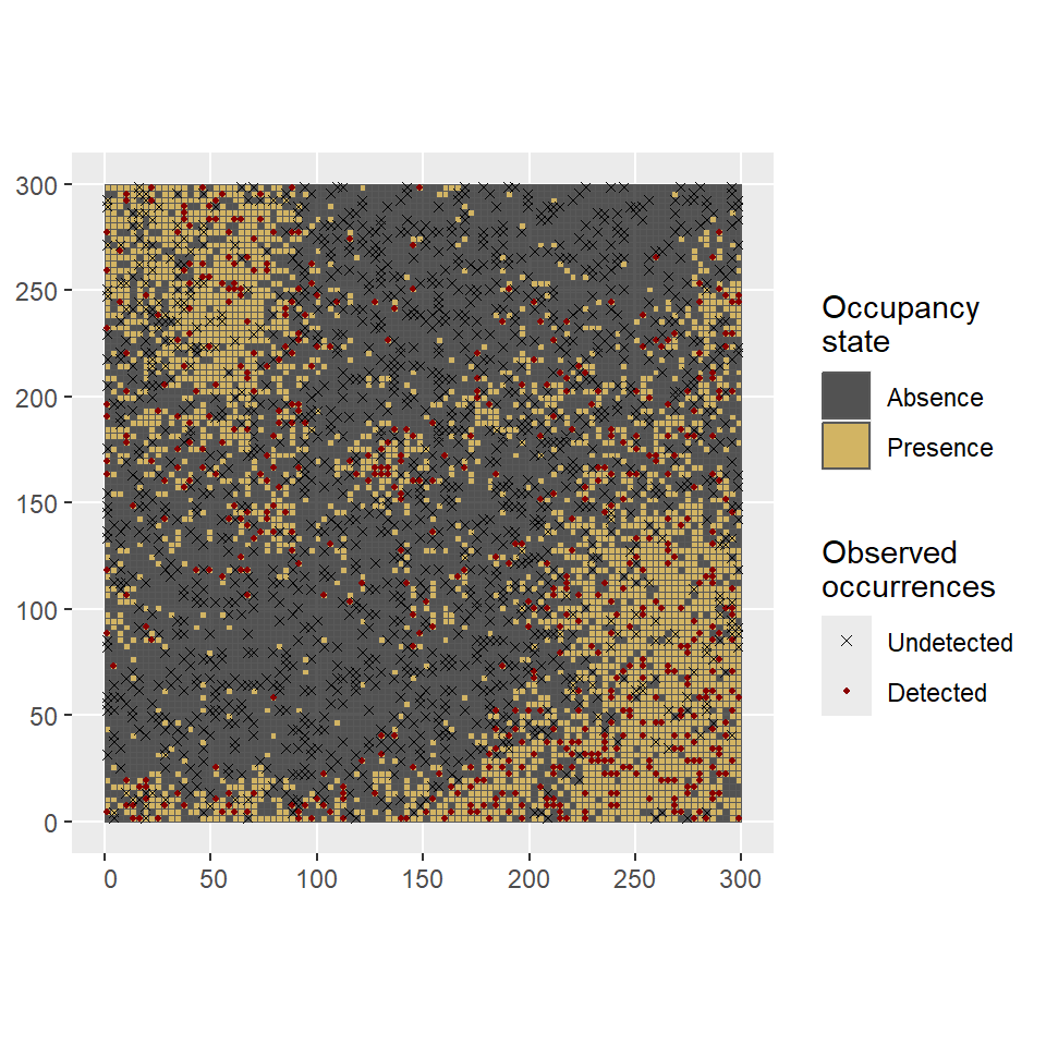
Figure 3: Simulated occupancy probabilities and true presence/absence state

2.2 Observational process model sub-component

Firs, a random sample of 20 % of the total cells is obtained.

Code

# number of cells/sites in the sample
nsites = round(ncells*.20)
site_id = sample(1:ncells, size=nsites, replace=FALSE) # cell id
# add an indicator of whether a cell is in the sample or not
customGrid$sample <- ifelse(customGrid$cellid%in%site_id,1,0)

Then, we define model parameters \(\alpha\) , detection probabilities \(p\) and observed number of occurrences \(y\) across \(K=3\) visits per site/cell (Figure 4). Additionally, a survey-level covariate \(g_2\) is simulated at every surveyed cell to allow detection probabilities to vary by visit.

Code

# Number of vistis
K= 3
# Observational process model coeficcients
alpha <- c(NA,NA,NA)
alpha[1] <- qlogis(0.6) # Base line detection probability
alpha[2] <- 1 # detection covariate g1 effect
alpha[3] <- 0.5 # detection covariate g2 effect

# Survey-level detection covariate g2
g2 <- array(runif(n = nsites * K, -1, 1), dim = c(nsites, K))

# Detection probabilities and observed occurrences
# Create empty matrix to store the results
y <- p.mat <- matrix(NA,nrow = nsites,ncol=3) 

# loop over visits
for(j in 1:K){
 p.mat[,j] <- inla.link.logit(alpha[1] + 
                              alpha[2]*g_s[site_id] + 
                              alpha[3]*g2[, j], inverse = T)
 y[,j] <- rbinom(n = nsites,size = 1,prob = p.mat[,j]*z[site_id] )
}

Create data set Table 1:

Code

# centroid of the cell

Occ_data_1 <- customGrid %>%
  st_centroid() %>%
  filter(sample==1) %>%
  dplyr::select(-c('sample'))

Obs_data <- data.frame(y = y, # detectio/non-detection data
           g2 = g2, # survey level covariate
           cellid = site_id)

Occ_data_1 <- left_join(Occ_data_1,Obs_data,by = "cellid") 

# append coordinates as columns

Occ_data_1[,c('x.loc','y.loc')] <- st_coordinates(Occ_data_1)
Occ_data_1 = st_drop_geometry(Occ_data_1)
# Save CSV file for analysis
write.csv(Occ_data_1,file='Occ_data_1.csv',row.names = F)

Table 1: First 6 entries of the occupancy data

cellid	y.1	y.3	g2.1	g2.2	g2.3	x.loc	y.loc
2	0	0	0.5714531	0.3866185	-0.2529522	4.5	1.5
5	0	1	-0.1941702	-0.7073133	0.4481461	13.5	1.5
6	0	1	-0.3740240	0.9385314	-0.1100978	16.5	1.5
7	0	0	0.3056664	0.5610409	0.7647462	19.5	1.5
9	1	0	0.6081176	-0.4150512	0.1087413	25.5	1.5
23	0	0	0.1278117	-0.9585974	-0.9708703	67.5	1.5

Figure 4: Observed detection/non-detection records at sampled sites and true occupancy state.

3 Simulate space-time occupancy data

Here we simulate data for a space-time occupancy model by defining a SPDE for the spatial domain and an autoregressive model of order 1, i.e. AR(1), for the time component (this is separable space-time model where the spatio-temporal covariance is defined by the Kronecker product of the covariances of the spatial and temporal random effects, see (Cameletti et al. 2012) for more details).

We set a total of nT = 5 discrete time points where the occupancy state changes. We can use the book.rspde() function available in the spde-book-functions.R file (Krainski et al. 2018) to simulate \(t = 1,\ldots,nT\) independent realizations of the random field¹. Then, temporal correlation is introduced:

\[ \omega(s_i,t) = \rho \ \omega(s_i,t-1) + \epsilon(s_i,t), \]

where \(\pmb{\epsilon} \sim N(0,\Sigma = \sigma_{\epsilon}^2\tilde{\Sigma})\) are the spatially correlated random effects with Matérn correlation function \(\tilde{\Sigma}\) and \(\rho=0.7\) is the autoregressive parameter (\(\sqrt{1-\rho^2}\) is included so \(\omega(s_i,1)\) comes from a \(N(0,\Sigma/(1-\rho^2)\) stationary distribution; see (Cameletti et al. 2012)).

Code

# load helping functions

source('spde-book-functions.R')

# Time points
nT = 5
# parameters of the Matern


# Create a fine mesh
mesh_sim = fm_mesh_2d(loc.domain = st_coordinates(boundary_sf)[,1:2],
                        offset = c(-0.1, -.2),
                        max.edge = c(4, 50))
# Matern model
params <- c(sigma = sigma_spde, range = range_spde)

# generate samples from the random field

epsilon.t <- book.rspde(coord_grid, range = params[2], seed = seed,
                  sigma = params[1], n = nT, mesh = mesh_sim,
                  return.attributes = TRUE)

# temporal dependency
rho <- 0.65

omega_st <- epsilon.t

for (t in 2:nT){
  omega_st[, t] <- rho * omega_st[, t - 1] + sqrt(1 - rho^2) * epsilon.t[, t]
}

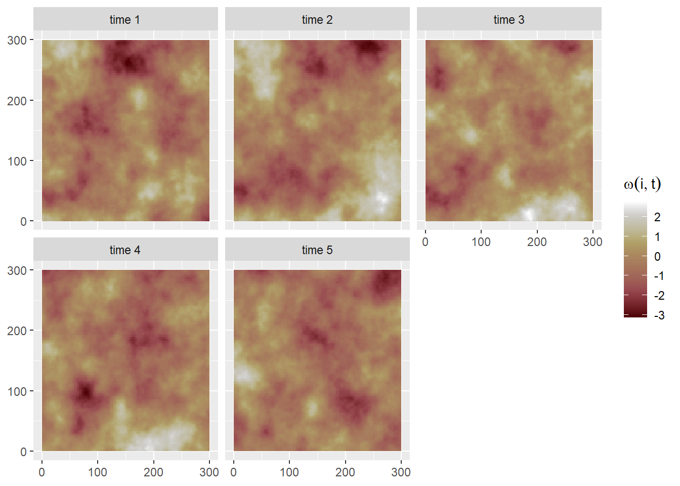
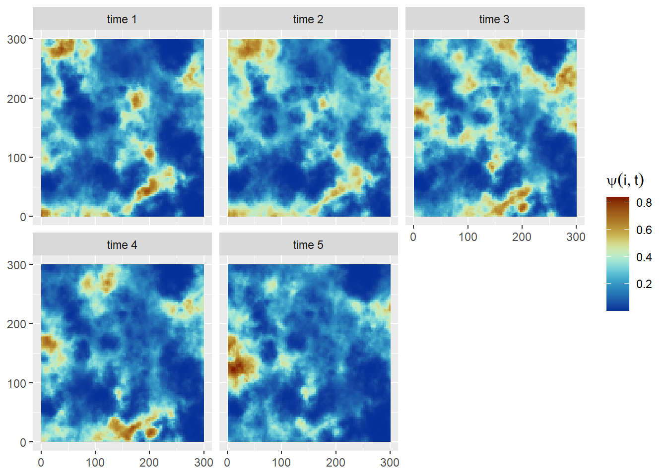
Figure 5: simulated spatio-temporal Gaussian field

Then we can simulate the occupancy state of cell \(i\) at time \(t\) (Figure 6) as follows:

\[\begin{align}z_{it}&\sim \mathrm{Bernoulli}(\psi_{it})\nonumber\\\mathrm{logit}(\psi_{it}) &= \beta_0 + \beta_1 x^2_i + \omega_{it}.\end{align}\]

Code

# State process model coeficcients
beta <- c(NA,NA)
beta[1] <- -0.5
beta[2] <- - 1 

z.mat = psi.mat = matrix(NA,ncol=nT,nrow=dim(coord_grid)[1])

for(t in 1:nT){
  # Occupancy probabilities
  psi.mat[,t] = inla.link.logit(beta[1] + beta[2]*x_s^2 + omega_st[,t], inverse = T)
  # True occupancy state
  z.mat[,t] <- rbinom(ncells, size = 1, prob = psi.mat[,t])
}

Figure 6: Simulated occupancy probabilities

Species detection/non-detection data at site \(i\) during visits \(j\) and time \(t\) is simulated from:

\[\begin{align} y_{ijt} &\sim \mathrm{Bernoulli}(p_{ijt} \times z_{it})\\ p_{ijt} &= \alpha_0 + \alpha_1 g_{ijt}\\ \end{align}\]

Detection probabilities vary over space, time and survey through a simulated covariate \(g_{ijt}\). Often, locations are not surveyed regularly, resulting in unbalanced sampling scenarios. To simulate this, we introduce missing values with a constant probability for each site \(\times\) time \(\times\) survey combination. This missing values represent locations that were not surveyed on a given occasion.

Code

# Max number of vistis
K= 3
# Observational process model coeficcients
alpha <- c(NA,NA)
alpha[1] <- qlogis(0.3) # Base line detection probability
alpha[2] <- -1.5 # detection covariate effect

# Survey-level detection covariate g.t
g.t <- array(runif(n = nsites * K * nT, -1, 1), dim = c(nsites, K, nT))

# Observed data

# matrices to store each site x survey combination
y_mat <- p_mat <- matrix(NA,nrow = nsites,ncol=K)
colnames(y_mat) < paste("y",1:K,sep="")

logical(0)

Code

# empty list for storing  each detection at each time point
y.t <- list()

# Constant NA probability
missing.p <- 0.1

# Detection/nondetection data (i.e. observed presence/absence records)
for(t in 1:nT){
  for(j in 1:K){
    p_mat[,j] <- inla.link.logit(alpha[1] + 
                                   alpha[2]*g.t[,j,t],
                                   inverse = T)
    y_mat[,j] <- rbinom(n = nsites,
                        size = 1,
                        prob = z.mat[site_id,t] * p_mat[,j])
    turnNA <- rbinom(nsites, 1, missing.p)
    y_mat[,j] <- ifelse(turnNA == 1, NA, y_mat[,j])
  }
  y.t[[t]] <-  y_mat
}

Finally, create and save data set.

Code

Obs_data.t <- do.call("rbind",y.t) %>% data.frame() %>%
  bind_cols(apply(g.t,2L,c))
colnames(Obs_data.t) <- c(paste("y",1:K,sep=""),paste("g",1:K,sep=""))

Obs_data.t <- Obs_data.t %>%
  mutate(cellid= rep(site_id,nT),time=rep(1:nT,each=nsites))

# centroid of the cell
Occ_data_2 <- suppressWarnings(customGrid %>%
                                 st_centroid()) %>%
  filter(sample==1) %>%
  dplyr::select(-c('sample'))


Occ_data_2 <- left_join(Occ_data_2,Obs_data.t,by = "cellid")

# append coordinates as columns
Occ_data_2[,c('x.loc','y.loc')] <- st_coordinates(Occ_data_2)
Occ_data_2 = st_drop_geometry(Occ_data_2)

# Save CSV file for analysis
write.csv(Occ_data_2,file='Occ_data_2.csv',row.names = F)

4 Spatially varying coefficients (SVC)

Here we simulate from a spatially varying coefficient model by adopting a space model with Matérn spatial covariance and a AR(1) time component. The same setting described for the space-time model will be used to drawn independent realization from the random field by using the book.rMatern()function. Then, temporal autocorrelation will be introduced to the dynamic regression coefficient \(\beta_t\) through the AR(1) structure described in the previous section (Note: The term \((1 - \rho^2)\) is added because of INLA internal AR(1) model parametrization; (Krainski et al. 2018)).

Code

# realization of the random field
set.seed(seed)
beta_1 <- book.rMatern(nT, coord_grid, range = range_spde,
                      sigma = sigma_spde)

# introduce temporal correlation
beta_1[, 1] <- beta_1[, 1] / (1 - rho^2)

for (t in 2:nT) {
  beta_1[, t] <- beta_1[, t - 1] * rho + beta_1[, t] *
    (1 - rho^2)
}

Occupancy probabilities (Figure 7) are then defined on the logit scale as:

\[ \mathrm{logit}(\psi_{it}) = \beta_0 + \beta_{1}(i)t + \omega(i) \]

where \(\omega(i)\) is the same field defined for the simple spatial occupancy model (Section 2). The detection probabilities and observed occurrences are simulated in the same way as in Section 3.

Code

set.seed(seed)

# intercept and mean of the effect
beta0 <- -1

z.mat = psi.mat = matrix(NA,ncol=nT,nrow=dim(coord_grid)[1])

scale_t <- scale(1:nT) %>% c()

for(t in 1:nT){
  # Occupancy probabilities
  psi.mat[,t] = inla.link.logit(beta0 + beta_1[,t]*scale_t[t] + omega_s, inverse = T)
  # True occupancy state
  z.mat[,t] <- rbinom(ncells, size = 1, prob = psi.mat[,t])
}


# Max number of vistis
K= 3
# Observational process model coeficcients
alpha <- c(NA,NA)
alpha[1] <- qlogis(0.3) # Base line detection probability
alpha[2] <- -1.5 # detection covariate effect

# Survey-level detection covariate g2
g.t <- array(runif(n = nsites * K * nT, -1, 1), dim = c(nsites, K, nT))


# matrices to store each site x survey combination
y_mat <- p_mat <- matrix(NA,nrow = nsites,ncol=K)

# empty list for storing  each detection at each time point
y.t <- list()

# Constant NA probability
missing.p <- 0.1

# Detection/nondetection data (i.e. observed presence/absence records)
for(t in 1:nT){
  for(j in 1:K){
    p_mat[,j] <- inla.link.logit(alpha[1] + 
                                   alpha[2]*g.t[,j,t],
                                   inverse = T)
    y_mat[,j] <- rbinom(n = nsites,
                        size = 1,
                        prob = z.mat[site_id,t] * p_mat[,j])
    turnNA <- rbinom(nsites, 1, missing.p)
    y_mat[,j] <- ifelse(turnNA == 1, NA, y_mat[,j])
  }
  y.t[[t]] <-  y_mat
}


Obs_data.t <- do.call("rbind",y.t) %>% data.frame() %>%
  bind_cols(apply(g.t,2L,c))
colnames(Obs_data.t) <- c(paste("y",1:K,sep=""),paste("g",1:K,sep=""))

Obs_data.t <- Obs_data.t %>%
  mutate(cellid= rep(site_id,nT),time=rep(1:nT,each=nsites))


# centroid of the cell
Occ_data_3 <- suppressWarnings(customGrid %>%
                                 st_centroid()) %>%
  filter(sample==1) %>%
  dplyr::select(-c('sample'))


Occ_data_3 <- left_join(Occ_data_3,Obs_data.t,by = "cellid")

# append coordinates as columns
Occ_data_3[,c('x.loc','y.loc')] <- st_coordinates(Occ_data_3)
Occ_data_3 = st_drop_geometry(Occ_data_3)


# Save CSV file for analysis

write.csv(Occ_data_3,file='Occ_data_3.csv',row.names = F)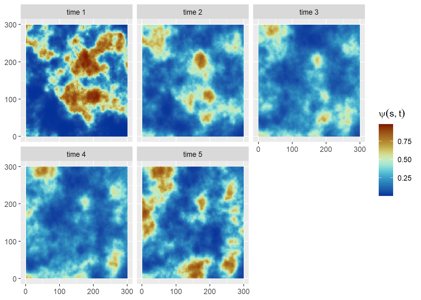

Figure 7: Simulated occupancy probabilities from a SVC model

References

Cameletti, Michela, Finn Lindgren, Daniel Simpson, and Håvard Rue. 2012. “Spatio-Temporal Modeling of Particulate Matter Concentration Through the SPDE Approach.” AStA Advances in Statistical Analysis 97 (2): 109–31. https://doi.org/10.1007/s10182-012-0196-3.

Krainski, Elias, Virgilio Gómez-Rubio, Haakon Bakka, Amanda Lenzi, Daniela Castro-Camilo, Daniel Simpson, Finn Lindgren, and Håvard Rue. 2018. Advanced Spatial Modeling with Stochastic Partial Differential Equations Using r and INLA. Chapman; Hall/CRC. https://doi.org/10.1201/9780429031892.

Footnotes

Note: If you are using INLA development version you might need modify the book.rspde function. Specifically, change the inla.mesh.project function to fmesher::fm_evaluator function to project the mesh into the domain coordinates.↩︎