install.packages("INLA",
        repos=c(getOption("repos"),
INLA="https://inla.r-inla-download.org/R/testing"), dep=TRUE)Fitting Occupancy models with R-INLA
This section describes the steps to fit occupancy models in R-INLA using simulated data (simulation details can be found in the Data Simulation tab).
Make sure you have that latest R and R-INLA versions installed:
Rversion4.4.0or above-
R-INLAversionINLA_24.06.04or above. For latest testing version use:
1 Simple Spatial Occupancy Model
The following simple spatial occupancy model is fitted to the simulated data:
\[\begin{align} z_{i} &\sim \mathrm{Bernoulli}(\psi_{i})~~~\mbox{for } i=1,\ldots,M_{sites} \nonumber \\ \mathrm{logit}(\psi_{i}) &= \beta_0 + \beta_1 x_i + \omega_i \nonumber \\ y_{ij}|z_{i} &\sim \mathrm{Bernoulli}(z_{i} \times p_{ij})\nonumber\\ \mathrm{logit}(p_{ij}) &= \alpha_0 + \alpha_1 g_{1i} + \alpha_2 g_{2ij}. \label{eq:SSOM} \end{align}\]Here, \(z\) denotes the occupancy state with occupancy probabilities \(\psi\) defined on the logit scale as a linear function of the simulated covariate \(x\) with unknown parameters \(\beta_0\) (Intercept), \(\beta_1\) (slope) and \(\omega\) (a spatial Gaussian random field describing the spatial structure in the data).
The response \(y\) is the detection/non-detection data given \(z\) , and the detection probabilities \(p\) are defined on the logit scale as a linear function of simulated covariates \(g_1\) and \(g_2\) with unknown parameters \(\alpha_0\) (Intercept) and \(\alpha_1\) , \(\alpha_2\) (slopes).
1.1 Set up
We first load the data and prepare it in the format that is required by R-INLA.
Code
library(INLA)
library(inlabru)
library(fmesher)
library(tidyverse)
library(sf)
library(terra)
library(dplyr)


occ_data <- read.csv("Occ_data_1.csv")
x_covariate <- terra::rast('raster data/x_covariat.tif')
g_covariate <- terra::rast('raster data/g_covariat.tif')

# Extract the covariate values

# Convert to sf and evaluate site-level covariates at each cell

SSOM_sf = occ_data %>%
  st_as_sf(coords = c('x.loc','y.loc'))

SSOM_sf = SSOM_sf %>%
  dplyr::select(-cellid) %>%
        mutate(terra::extract(x_covariate,st_coordinates(SSOM_sf)),
               terra::extract(g_covariate,st_coordinates(SSOM_sf)))


# append coordinates and remove geometry attributes

SSOM = SSOM_sf %>%
    mutate(x.loc= st_coordinates(SSOM_sf)[,1],
           y.loc= st_coordinates(SSOM_sf)[,2]) %>%
st_drop_geometry()| y.1 | y.2 | y.3 | g2.1 | g2.2 | g2.3 | x_s | g_s | x.loc | y.loc |
|---|---|---|---|---|---|---|---|---|---|
| 0 | 0 | 0 | 0.57 | 0.39 | -0.25 | 0.25 | -0.67 | 4.5 | 1.5 |
| 0 | 0 | 1 | -0.19 | -0.71 | 0.45 | 0.79 | -0.91 | 13.5 | 1.5 |
| 0 | 0 | 1 | -0.37 | 0.94 | -0.11 | 0.77 | -0.97 | 16.5 | 1.5 |
| 0 | 0 | 0 | 0.31 | 0.56 | 0.76 | 0.88 | -1.12 | 19.5 | 1.5 |
| 1 | 0 | 0 | 0.61 | -0.42 | 0.11 | 0.69 | -1.23 | 25.5 | 1.5 |
| 0 | 0 | 0 | 0.13 | -0.96 | -0.97 | 0.99 | -0.58 | 67.5 | 1.5 |
To better understand the data structures that are used by R-INLA, we will split the data as follows:
-
The observed presence/absence matrix \(Y_{M\times K}\) with binary entries \(y_{ij}\) for \(i \in 1,\ldots M\) sites and \(j \in 1,\ldots,K\) maximum number of visits.
-
A matrix for the spatial coordinates of the sites
-
The occupancy covariates for the state/occupancy process.
-
The detection covariates for the observational process declared as a matrix \(G_{M \times \left[ K (P+1)\right]}\), where \(P\) is the number of detection covariates. Here, the first \(P+1\) columns correspond to the intercept (1st column) and the \(l= 1,\ldots,P\) covariates \(g_{ijl}\) on the first visit \(j =1\) across \(i = 1,\ldots,M\) sites. A new intercept column defines the next \(l\) covariates measurements at the second visit \(j=2\) , and so on until the \(K\)th visit.
 Important
For constant detection probabilities a \(G_{M \times \left[ K (P+1)\right]}\) matrix with \(g_{ijl} = 1 \ \forall\ (i,j,l)\) entries must be specified. Likewise if a site-level covariate is to be used, then the values for that covariate must be repeated across the \(K\) maximum number of visits. The function
inla.Occupancy_detCovbelow helps farmating the detection data as required byR-INLA. It receives as arguments either (i) a \(G_{ij}\) matrix for a single covariate input or (ii) a list \(G^{(l)}_{ij}\) where the \(l-\)th element of the list corresponds to the \(l-\)th survey or site level covariate:Code
inla.Occupancy_detCov <- function(X_det){ if(class(X_det)=="list"){ if(length(X_det)>10){ warning("exceeded number of detection covariates, numerical issues may occur") } if(lapply(X_det, ncol)%>%unlist()%>%unique()%>%length()>2){ stop("inconsistent number of visits in provided detection covariates") } if(length(lapply(X_det, nrow) %>% unlist() %>% unique())>1){ stop("inconsistent number of sites in provided detection covariates") } K<- lapply(X_det, ncol) %>% unlist() %>% max() # Max num of visits M<- lapply(X_det, nrow) %>% unlist() %>% unique() # Number of sites P <- length(X_det) if(lapply(X_det, ncol)%>%unlist()%>%unique()%>%length()==2 & 1 %in% lapply(X_det, ncol)%>%unlist()%>%unique()){ warning(paste("At least one covariate of dimension [",M,",1] has been provided, values for this covariate will be repeated over the max numver of visits",sep="")) for(l in which(lapply(X_det, ncol) %>% unlist() < K)){ X_det[[l]] <- do.call("cbind",replicate(K,X_det[[l]])) } } covariates <- do.call("cbind", lapply(1:K, function(i) { do.call("cbind", lapply(X_det, function(mat) mat[, i])) })) } if(is.data.frame(X_det)|is.matrix(X_det)){ K<- ncol(X_det) M<- nrow(X_det) P <- 1 covariates <- as.matrix(X_det) } X_mat <- matrix(NA,nrow=M,ncol=K*(P+1)) X_mat[,seq(1,(K*(P+1)),by=(P+1))]<-1 # add Intercept at the begining of each visit-specific covariate matrix X_mat[, which(!(1:(K*(P+1)) %in% seq(1,(K*(P+1)),by=(P+1))))] <- covariates return(X_mat) }Table 2: First 6 entries of the detection covariate g as required by R-INLA. Visit 1 Visit 2 Visit 3 Intercept g1. g2,1 Intercept g1. g2,2 Intercept g1. g2,3 1.00 −0.67 0.57 1.00 −0.67 0.39 1.00 −0.67 −0.25 1.00 −0.91 −0.19 1.00 −0.91 −0.71 1.00 −0.91 0.45 1.00 −0.97 −0.37 1.00 −0.97 0.94 1.00 −0.97 −0.11 1.00 −1.12 0.31 1.00 −1.12 0.56 1.00 −1.12 0.76 1.00 −1.23 0.61 1.00 −1.23 −0.42 1.00 −1.23 0.11 1.00 −0.58 0.13 1.00 −0.58 −0.96 1.00 −0.58 −0.97
1.1.1 Constructing the mesh and defining the SPDE
The linear predictor can include a variety of random effects such as smooth terms or spatiotemporal components by incorporating Gaussian random fields (GRFs) into models. This is achieved by using the stochastic partial differential equation (SPDE) method introduced by Lindgren, Rue, and Lindström (2011). The SPDE approach relies discretizing the space by defining a mesh that creates an artificial set of neighbours over the study area that allows for the spatial autocorrelation between observation to be calculated. How the mesh is constructed will have an important impact on the inference and predictions we make. Thus, it is important to create a good mesh to ensure results are not sensible to the mesh itself (guidance for creating a mesh can be found in Krainski et al. (2018) section 2.6.3). The inla.spde2.pcmatern() function is used to define the SPDE model. Using the penalized complexity (PC) priors derived in Fuglstad et al. (2018) on the range and marginal standard deviation.
Code
boundary_sf = st_bbox(c(xmin = 0, xmax = 300, ymax = 0, ymin = 300)) %>%

  st_as_sfc() %>% st_as_sf()

mesh = fm_mesh_2d(loc.domain = st_coordinates(boundary_sf)[,1:2],

                    offset = c(-0.1, -.2),

                    max.edge = c(15, 30))

matern <- inla.spde2.pcmatern(mesh,

                              prior.range = c(100, 0.5),

                              prior.sigma = c(1, 0.5))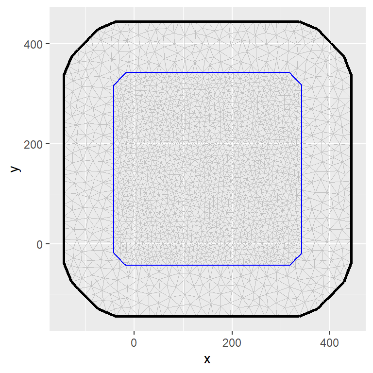
To define a spatial model we create the projector A matrix that maps the spatial Gaussian random field to the locations of the observed data and organize it along with the data, indeces and covariates.
Typically, this is done through the inla.stack() function (see Krainski et al. (2018) sections 2.3.2 and 2.3.3 for more details). However, recent developments in R-INLA allows the mapping matrix A to be called directly in the model formula to facilitate the specification of spatial models through the A.local argument.
Here, we present how these two approaches can be implemented. However, since the later feature is still under development, we encourage practicioners to use the inla.stack() function for now.
When building the stack we need to supply three main arguments:
List containing the data and the detection covariates matrix,
List of projector matrices (in this case the projector matrix A for the spatial field and a matrix that maps the covariate and the response)
List of effects including (i) the occupancy intercept, (ii) the index set for the spatial field (that takes into account the number of mesh points in the SPDE ) and (iii) a list of the site-level covariate(s) for the state process of interest.
# projector matrix A

A_sp <- inla.spde.make.A(mesh = mesh,loc = XY_coords)

# index set

iset_sp <- inla.spde.make.index(name = "spatial_field", matern$n.spde)


# build the stack
stk <- inla.stack(data=list(Y = Y_mat,  # observed occurrences
                            X = X_det), # detection covariate
                     A=list(A_sp,1),        # project matrices
                  effects=list(iset_sp,     # the spatial index
                     data.frame(Int_occ=1,  # Occ Intercept
                     occ_cov = X_occ$x_s)), # covariate x
                  #this is a quick name so yo can call upon easily
                  tag='ssom')
Now we define the model components (left hand side -observational model components; right hand side - state process components) and fit the model using the inla function:
formula_ssom <- inla.mdata(Y,X) ~  -1 +  Int_occ +
  occ_cov +  f(spatial_field, model=matern)

model_ssom <- inla(formula_ssom, # model formula

                 data=inla.stack.data(stk), # data stack

                 family= 'occupancy', # model likelihood

                 # priors

                 control.fixed =  list(prec = 1/2.72, prec.intercept = 1/2.72),

                 # matrix of predictors

                 control.predictor=list(A=inla.stack.A(stk),compute=TRUE),

                 # compute WAIC and DIC

                 control.compute = list(dic = TRUE, waic = TRUE, config = TRUE),

                 verbose = FALSE,

                 # choose link functions for:

                 # (i) the state process (control.link)

                 # (ii) the observation process (link.simple)

                 control.family = list(control.link = list(model = "logit"),

                                       link.simple = "logit",

                 # priors for hyperparameters

                 hyper = list(
                  # Detection intercept prior
                   beta1 = list(param = c(0,1), initial = -1),
                  # Covariate 1 effect prior
                   beta2 = list(param = c(0,1/2.72)),
                  # Covariate 2 effect prior
                   beta3 = list(param = c(0,1/2.72))

                 )

))We explicitly removed the intercept in the occupancy formula and included it as covariates in the list of effects. Then, the covariate terms (which are now included in the projector matrix) are passed on to inla() through the control.predictor argument. Priors for the detection parameters are provided as a list in the hyper option of the control.family argument. The order of these priors matches the order of the detection covariates in the matrix supplied in the inla.mdata argument.
Compute the mapping matrix A using the inla.spde.make.Afunction which receives as arguments the mesh and the data coordinates. Then, the occupancy data need to be changed slightly by explicitly adding (1) the intercept term as a column of 1’s, and (2) an empty vector for spatial field (as this will be passed on directly to the f() function in inla).
Then, we can supply the data as a list containing the following elements:
A list of the occupancy covariates including the intercept (note that the names of the elements of this list are the ones that should be specified in the model formula).
Detection/non-detection data \(Y_{M\times K}\).
Detection covariates matrix \(G_{M \times \left[ K (P+1)\right]}\).
Code
data_list = as.list(X_occ2)
data_list$Y = Y_mat
data_list$X = X_det
Now, we define the model components (left hand side -observational model components; right hand side - state process components) and fit the model using the inla function:
formula_ssom <- inla.mdata(Y,X) ~  -1 + Int_occ +
  occ_cov +  f(spatial_field, model=matern,  A.local = A_sp)

model_ssom <- inla(formula_ssom,    # model formula
                 data= data_list,        # data
                 family= 'occupancy', # model likelihood

                 # priors
                 control.fixed =  list(prec = 1/2.72, prec.intercept = 1/2.72),

                 # compute WAIC and DIC
                 control.compute = list(dic = TRUE, waic = TRUE, config = TRUE),
                 verbose = FALSE,

                 # choose link functions for:

                 # (i) the state process (control.link)
                 # (ii) the observation process (link.simple)
                 control.family = list(control.link = list(model = "logit"),
                                        link.simple = "logit",

                 # priors for hyperparameters
                 hyper = list(
                   # Detection intercept prior
                   beta1 = list(param = c(0,1), initial = -1),
                   # Covariate 1 effect prior
                   beta2 = list(param = c(0,1/2.72)),
                   # Covariate 2 effect prior
                   beta3 = list(param = c(0,1/2.72))
                 )
                 ))
Priors for the detection parameters are provided as a list in the hyper option of the control.family argument. The order of these priors matches the order of the detection covariates in the matrix supplied in the inla.mdata argument.
1.2 Results
The summary of the fixed effect, namely \(\beta_0\) and \(\beta_1\) can be retrieved from model_ssom$summary.fixed while detection parameters \(\alpha_0\) and \(\alpha_1\) are contained, along with the range and standard deviation, in model_ssom$summary.hyperpar.
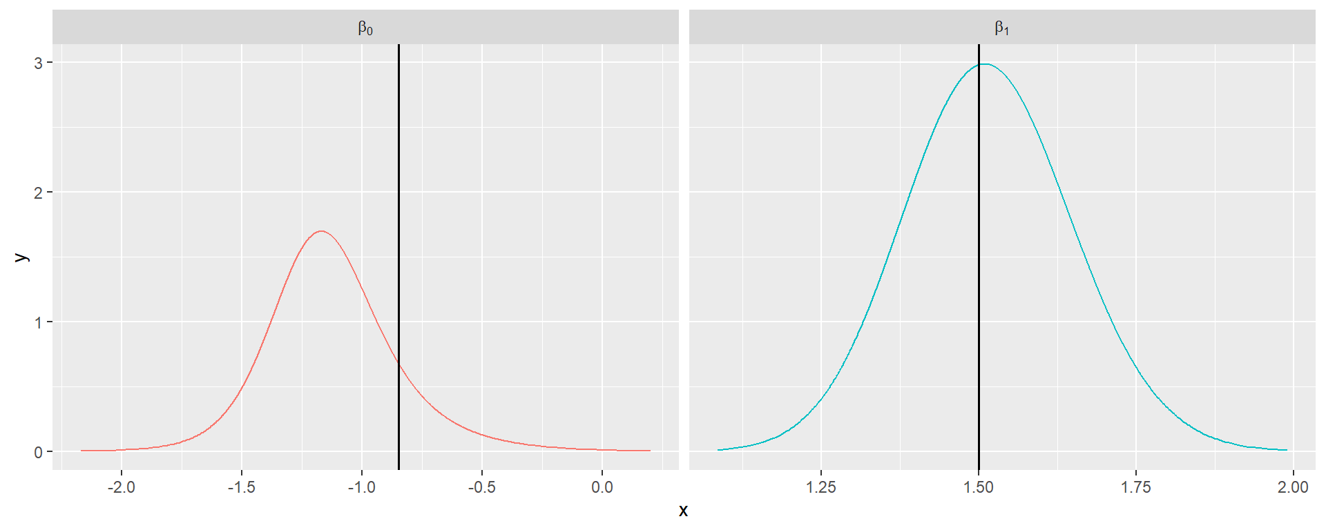
Summary results from the fitted SSOM are shown in Table 3 and posterior densities on Figure 1.
| par | true | mean | quant0.025 | quant0.975 |
|---|---|---|---|---|
| \(\beta_0\) | -0.85 | -1.12 | -1.63 | -0.48 |
| \(\beta_1\) | 1.50 | 1.51 | 1.26 | 1.78 |
| \(\alpha_0\) | 0.41 | 0.43 | 0.31 | 0.55 |
| \(\alpha_1\) | 1.00 | 0.98 | 0.86 | 1.11 |
| \(\alpha_2\) | 0.50 | 0.58 | 0.39 | 0.76 |
| \(\rho\) | 100.00 | 95.34 | 40.15 | 201.71 |
| \(\sigma\) | 1.00 | 0.77 | 0.52 | 1.10 |
1.3 Model comparison through cross-validation
Next we introduce how to implement modelling comparison using leave-out group cross validation (LGOCV). The underlying idea is that of a Bayesian prediction setting where we approximate the posterior predictive density \(\pi(\mathbf{\tilde{Y}}|\mathbf{y})\) defined as the integral over the posterior distribution of the parameters, i.e.
\[ \pi(\mathbf{\tilde{Y}}|\mathbf{y}) = \int_\theta \pi(\mathbf{\tilde{Y}}|\theta,\mathbf{y}) \pi(\theta|\mathbf{y})d\theta \]
the LGOCV selects a fixed test point \(i\) and remove a certain group of data \(\mathbb{I}_i\) according to a specific prediction task. Thus, we are interested in the posterior predictive density
\[ \pi(Y_i|\mathbf{y}{-\mathcal{I}i}) = \int\theta \pi(Y_i|\theta,\mathbf{y}{-\mathbb{I}_i}) \pi(\theta|\mathbf{y})d\theta \]
With this, a point estimate \(\tilde{Y_i}\) can be computed based on \(\pi(Y_i|\mathbf{y}_{-\mathbb{I}_i})\) and the predictive performance be assessed using an appropriate scoring function \(U(\tilde{Y}_i,Y_i)\), for example, the log-score function
\[ \frac{1}{n}\sum_{i=1}^n \mathrm{log}~ \pi(\mathbf{\tilde{y}}|\mathbf{y}). \]
In this example, the LGOCV strategy will be used to compare the previous fitted spatially explicit occupancy model against a simple model that only considers a site iid random effect (note that since no structured spatial effect is being included, the data can be passed on to inla() as a list without the need for a stack).
SSOM_simple = as.list(data.frame(site= 1:nrow(SSOM),Int_occ = 1))
SSOM_simple$Y <- Y_mat
SSOM_simple$X <- X_det

formula_simple = inla.mdata(Y,X)  ~ f(site, model =  "iid")

model_simple <- inla(formula_simple, data=SSOM_simple,
                     family= 'occupancy',verbose = FALSE,
               control.compute = list( config = TRUE,dic  = T, waic = T),
               control.fixed = list(prec.intercept = 1/2.72,prec = 1/2.72),
               control.family = list(control.link = list(model = "logit"),
                                     link.simple = "logit",
                                     hyper = list(beta1 = list(param = c(0,1),
                                                           initial = 0),
                                                  beta2 = list(param = c(0,1)),
                                                  beta3 = list(param = c(0,1))
                                                  )))
Warning in normalizePath(path.expand(path), winslash, mustWork):
path[1]="C:/Users/jaf_i/AppData/Local/Temp/Rtmp4wvNAp/file128a8554cbb1": The
system cannot find the file specifiedIn this example the leave-out group \(\mathbb{I}_i\) is manually defined for the \(i\)th row of the data based on a buffer of size \(b=25\) centered at each data point (we will use the sf object created before):
# create buffer of size 25 centred at each site
buffer <- st_buffer(SSOM_sf, dist = 25)

# Lists of the indexes of the leave-out-group for each observation i
Ii <- st_intersects(SSOM_sf,buffer)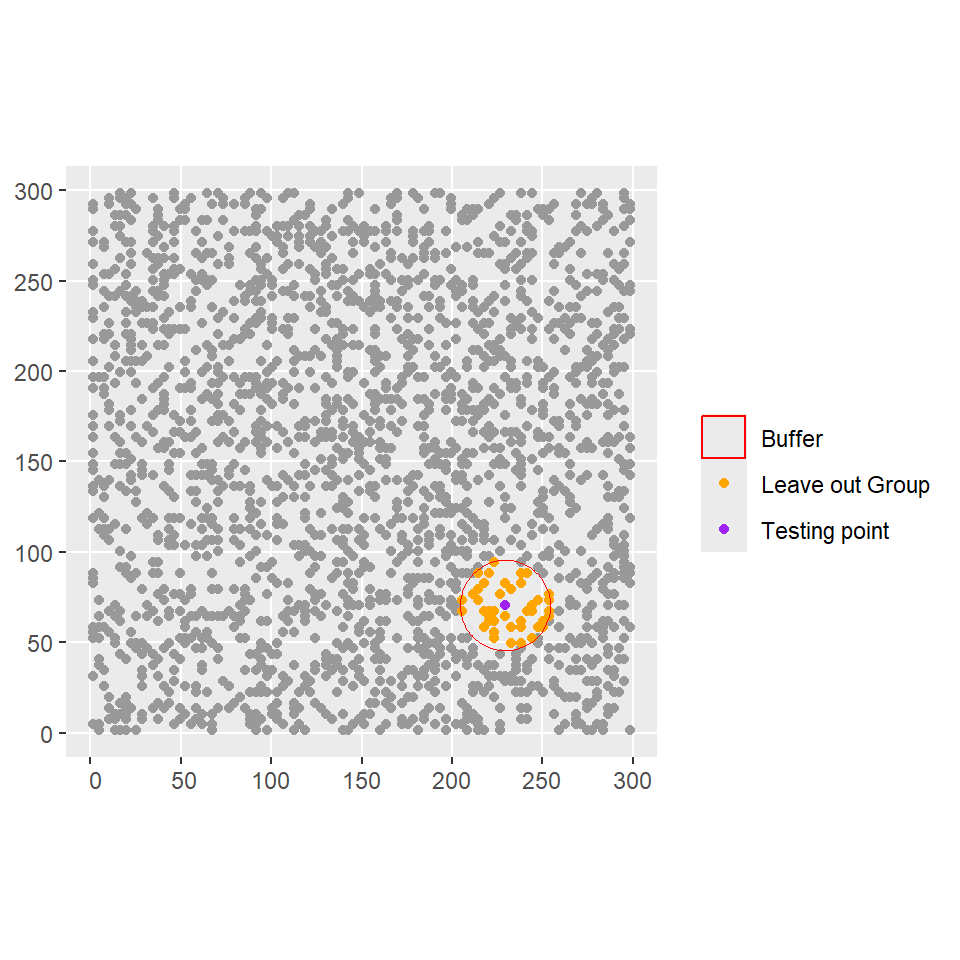
The LGOCV is used to evaluate the predictive performance of each model and the log-scores are computed as shown in Table 4.
lgocv_ssom = inla.group.cv(result = model_ssom, groups= Ii)
lgocv_simple = inla.group.cv(result = model_simple, group.cv = lgocv_ssom)

log_score_ssom <- mean(log(lgocv_ssom$cv),na.rm=T)
log_score_simple <-mean(log(lgocv_simple$cv),na.rm=T)| Log-Score LGOCV | |
|---|---|
| Continuous spatial Gaussian field |
Site iid random effect |
| −0.96 | −1.09 |
2 Spacetime Occupancy Models
Next, we illustrate how the following spatiotemporal occupancy model can be fitted using INLA:
\[\begin{align} z_{it} &\sim \mathrm{Bernoulli}(\psi_{it}) \nonumber \\ \mathrm{logit}(\psi_{it}) &= \beta_0 + f_1(\mbox{x}_i) + \omega(i,t) \nonumber \\ y_{ijt}|z_{it} &\sim \mathrm{Bernoulli}(z_{it} \times p_{ijt})\nonumber\\ \mathrm{logit}(p_{ijt}) &= \alpha_0 + \alpha_1 \mbox{g}_{ijt}. \label{eq:occ_model2} \end{align}\]The structure of this model is similar to the simple spatial occupancy model, with the main difference being that occupancy probabilities vary on space and time according to \(f_1(x_i)\) a smooth effect of the covariate \(x\) and \(\omega(i,t)\), a space-time Gaussian spatial field with AR1 time component (we also simplified the detection sub-model slightly by incorporating a single survey-level covariate).
2.1 Set up
First, we need the data to have the correct structure with columns representing the observed occurrences, number of visits, the cell/site id, the site-level covariates, and the time points. An additional filtering is made to remove the locations that were not visited in a given time point.
Code
# read the data
space_time_data <- read.csv("Occ_data_2.csv")
# raster data
x_covariate <- terra::rast('raster data/x_covariat.tif')
# function for structuring detection covariates
source("detection_covariates_function.R")

# Convert to sf
space_time_data_sf <- space_time_data %>%
  st_as_sf(coords = c('x.loc','y.loc'))

# evaluate covariate at each cell

space_time_data_sf <- space_time_data_sf %>%
        mutate(site = as.factor(cellid),
               terra::extract(x_covariate,st_coordinates(space_time_data_sf)))

# (optional) if an i.i.d random effect by sites is to be used.
levels(space_time_data_sf$site) <- 1:nlevels(space_time_data_sf$site)

spat_data  = space_time_data_sf %>%
  dplyr::select(-cellid) %>%
  mutate(x.loc= st_coordinates(space_time_data_sf)[,1],
y.loc= st_coordinates(space_time_data_sf)[,2]) %>% st_drop_geometry()| y1 | y2 | y3 | g1 | g2 | g3 | time | site | x_s | x.loc | y.loc |
|---|---|---|---|---|---|---|---|---|---|---|
| 0 | 1 | 1 | -0.71 | 0.05 | -0.18 | 1 | 1 | 0.25 | 4.5 | 1.5 |
| 0 | 0 | 0 | -0.29 | -0.91 | 0.09 | 2 | 1 | 0.25 | 4.5 | 1.5 |
| 0 | NA | 0 | 0.44 | -0.31 | -0.97 | 3 | 1 | 0.25 | 4.5 | 1.5 |
| NA | 0 | 0 | -0.43 | 0.93 | 0.58 | 4 | 1 | 0.25 | 4.5 | 1.5 |
| NA | 0 | 0 | 0.95 | -0.98 | -0.97 | 5 | 1 | 0.25 | 4.5 | 1.5 |
| 0 | 0 | 0 | 0.47 | -0.19 | 0.05 | 1 | 2 | 0.79 | 13.5 | 1.5 |
For the estimation of the smooth effect, we can reduce the number of knots used in the estimation process by grouping the covariate \(x\) values into equal length intervals with the inla.group() function and appending these grouped values to the data.
At this point we will also create a data frame for prediction, containing the values of the binned covariates \(x\) for every time time point in the data.
nT <- length(spat_data$time %>% unique) # number of time points
ncells <- length(values(x_covariate$x_s)) # number of cells in the whole area

# scale and centre the covariate value in the data input

spat_data <- spat_data %>%
  mutate(scale_x_s = scale(x_s)  %>% c())

# prediction data frame

pred_df = data.frame(x = rep(crds(x_covariate)[,1],nT),
                     y = rep(crds(x_covariate)[,2],nT),
                     x_s = rep(as.vector(scale(values(x_covariate$x_s))),nT),
                     time = rep(c(1:nT), each= ncells))

# binned covariate values.

xx = inla.group(c(spat_data$x_s, pred_df$x_s),
                n = 35)

# append grouped covariate values to the input and prediction data sets

spat_data$group_xs = xx[1:dim(spat_data)[1]]
pred_df$group_xs = xx[-c(1:dim(spat_data)[1])]
2.2 Fitting a space-time Occupancy model in INLA
To fit a separable space time model, the SPDE needs to be defined first:
boundary_sf = st_bbox(c(xmin = 0, xmax = 300, ymax = 0, ymin = 300)) %>%
  st_as_sfc() %>% st_as_sf()

mesh = fm_mesh_2d(loc.domain = st_coordinates(boundary_sf)[,1:2],
                    offset = c(-0.1, -.2),
                    max.edge = c(15, 30))

spde <- inla.spde2.pcmatern(mesh = mesh,
                              prior.range = c(100, 0.5),
                              prior.sigma = c(1, 0.5))
For building the projection matrix A, the coordinates and the time index need to be supplied. Again, we showcase how can this be done by either (1) constructing a data stack with the inla.stack() function or (2) by providing the projection matrix in the A.local argument.
To fit a separable space time model, the index set need to be defined (see Krainski et al. (2018) Section 7.1.2 for further reference on building the stack for a separable space time model in INLA). We can build the stack in a similar fashion to the one in Section 1.1.
# unique time points
t_points = unique(spat_data$time)

# index set; "spatialfield" is the name used in the model formula
iset_sp <- inla.spde.make.index(name = "spatialfield",
                                n.spde =  spde$n.spde,
                                n.group = length(t_points))

# projection matrix using the coordinates of the data and time index

A_sp <- inla.spde.make.A(mesh = mesh,
                         loc = as.matrix(spat_data[,c("x.loc","y.loc")]),
                         group = spat_data$time)

Y_mat <- spat_data %>%
  dplyr::select(num_range("y",1:3)) %>%
  as.matrix()
X_det <- spat_data %>%
  dplyr::select(num_range("g",1:3)) %>%
  inla.Occupancy_detCov()
X_cov <- spat_data %>%
  dplyr::select(c(time,site,group_xs))

stk <- inla.stack(data=list(Y = Y_mat,  X = X_det),
                  A=list(A_sp,1),
                  effects=list(c(list(Int_occ=1), #the Intercept
                                 iset_sp),  #the spatial index
                               #the covariates
                               as.list(X_cov)),
                  tag='spat')
Next we specify the prior for the temporal autoregressive parameter and the model formula:
# PC prior for the temporal autocorrelation
h.spec <- list(rho = list(prior = 'pc.cor0', param = c(0.5, 0.3)))

# extract unique values of the binned covariate
val_xs = sort(unique(xx))

formula_spat <- inla.mdata(Y,X) ~ -1 + Int_occ +
  f(group_xs, model = "rw2", values = val_xs)  +
   f(time, model = "iid") +
  f(spatialfield,
    model=spde,
    group = spatialfield.group,
control.group = list(model = 'ar1',hyper = h.spec))Notice that we have used the values argument when defining the rw2 effect to specify the values of the binned covariate at which we will like to do predictions (i.e., over the whole domain). Otherwise, the model would only look at the values of the binned covariate available in the data input.
Next we run the model (note that we have used Empirical Bayes integration strategy for computational purpose, see Gómez-Rubio (2020) for further details):
model_spat <- inla(formula_spat, #the formula
                   data=inla.stack.data(stk),  # the data stack
                   family= 'occupancy',   # model likelihood
                   control.fixed =  list(prec = 1, prec.intercept = 1),
                                     control.predictor=list(A=inla.stack.A(stk),
                                                            compute=TRUE),
                   control.compute = list(waic = TRUE,config = TRUE),
                      control.inla = list(int.strategy = "eb"),
                   #model diagnostics and config = TRUE gives you the GMRF
                   verbose = F,
                   control.family = list(control.link = list(model = "logit"),
                                         link.simple = "logit",
                            hyper = list(beta1 = list(param = c(0,1/3),
                                                              initial = 0),
                                         beta2 = list(param = c(0,1/3)))
                            ))
Warning in normalizePath(path.expand(path), winslash, mustWork):
path[1]="C:/Users/jaf_i/AppData/Local/Temp/Rtmp4wvNAp/file128a8460747": The
system cannot find the file specifiedTo define a separable space time model the projector matrix A of dimensions \([(M\times nT) \times (N \times nT)]\) (i.e. for \(nT\) times points, \(M\) sites, and \(N\) mesh nodes) needs to be specified by using the group argument which recieves the time index (i.e the different time points) for each observation in the dataset.
A_sp <- inla.spde.make.A(mesh = mesh,
                         loc = as.matrix(spat_data[,c("x.loc","y.loc")]),
                         group = spat_data$time)
Since we are not building a data stack, we can create a list containing the data we need to fit the model:
# Detection /non-detection data
Y_mat <- spat_data %>%
  dplyr::select(num_range("y",1:3)) %>%
  as.matrix()
# Detection covariates matrix
X_det <- spat_data %>%
  dplyr::select(num_range("g",1:3)) %>%
  inla.Occupancy_detCov()
# state process components:
# (i) grouped covariate
# (ii) time points
# (iii) intercept column of 1s
# (iv) empty vector for the spatial field.

X_cov <- spat_data %>%
  dplyr::select(c(time,group_xs)) %>%
  mutate(Int_occ = 1,
         spatialfield = rep(NA,nrow(spat_data)))

# Append to a list:
data_list <- as.list(X_cov)
data_list$Y <- Y_mat
data_list$X <- X_det
Next we specify the prior for the temporal autoregressive parameter and the model formula:
# PC prior for the temporal autocorrelation
h.spec <- list(rho = list(prior = 'pc.cor0', param = c(0.5, 0.3)))

# extract unique values of the binned covariate
val_xs = sort(unique(xx))

formula_spat <- inla.mdata(Y,X) ~ -1 + Int_occ +
  f(group_xs, model = "rw2", values = val_xs)  +
  f(time, model = "iid") +
  f(spatialfield,
    model=spde,
    A.local = A_sp,
    group = time,
control.group = list(model = 'ar1',hyper = h.spec))Notice that we have used the values argument when defining the rw2 effect to specify the values of the binned covariate at which we will like to do predictions (i.e., over the whole domain). Otherwise, the model would only look at the values of the binned covariate available in the data input.
Next we run the model (note that we have used Empirical Bayes integration strategy for computational purpose, see Gómez-Rubio (2020) for further details):
model_spat <- inla(formula_spat, # the formula
                   data=data_list,  # the data list
                   family= 'occupancy',
                   control.fixed =  list(prec = 1, prec.intercept = 1),
                   control.compute = list(waic = TRUE,config = TRUE),
                   control.inla = list(int.strategy = "eb"),
                   verbose = F,
                   control.family = list(control.link = list(model = "logit"),
                                         link.simple = "logit",
                           hyper = list(beta1 = list(param = c(0,1/3),
                                                     initial = 0),
                                        beta2 = list(param = c(0,1/3)))
                           ))
The posterior summaries (i.e. mean, quantiles, std.dev and mode) of the smooth term \(f(x)\) estimated using a RW2 are stored in model_spat$summary.random$group_xs. The estimated smooth term can then be plotted against the true function.
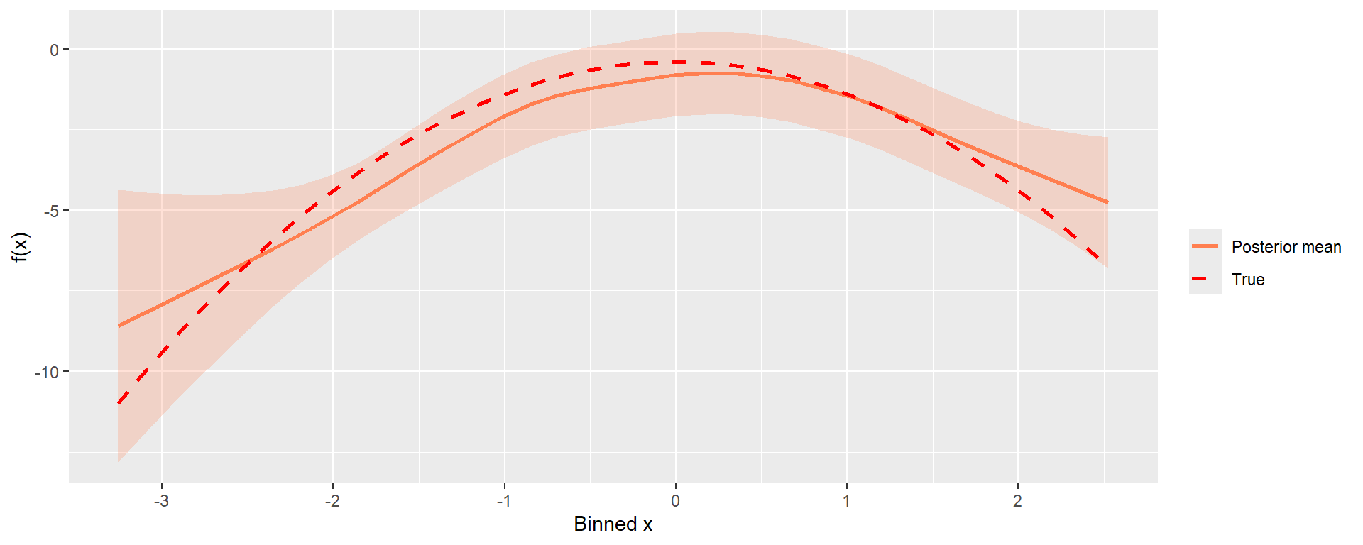
Model hyper parameters marginal densities can be accessed through model_spat$marginals.hyperpar, posterior summaries of such are shown in Table 5
| par | true | mean | quant0.025 | quant0.975 |
|---|---|---|---|---|
| \(\alpha_0\) | -0.85 | -0.86 | -0.96 | -0.76 |
| \(\alpha_1\) | -1.50 | -1.52 | -1.65 | -1.39 |
| practical range | 100.00 | 90.14 | 61.43 | 129.21 |
| \(\sigma\) | 1.00 | 0.84 | 0.70 | 1.01 |
| \(\rho\) | 0.65 | 0.49 | 0.27 | 0.68 |
2.3 Spatial predictions
In order to do predictions over space and time, we will need the prediction data set we created before, which contains the components used to fit the model. First, the projection matrix A is computed (this will be used for evaluating the model posterior samples of the Gaussian field in the next step).
A_spat = inla.spde.make.A(mesh= mesh, loc = cbind(pred_df$x, pred_df$y),
                        group = pred_df$time)
Then, posterior samples of the model will be drawn using the inla.posterior.sample() function. A function of the generated samples can be computed using the inla.posterior.sample.eval() function. To do so, we defined a function func_spat() to evaluate the linear predictor components on the posterior samples of the model.
samples_spat = inla.posterior.sample(1000, model_spat)

func_spat = function(...)

{
  eta = (Int_occ + group_xs[as.numeric(as.factor(pred_df$group_xs))] +
           (A_spat %*% spatialfield)[,1] +
          time[pred_df$time])
  eta

}

eval_samples = inla.posterior.sample.eval(func_spat, samples_spat)
Summaries of the posterior samples can then be appended to de prediction data frame for visualization (e.g., mean occupancy probabilities, linear predictor posterior mean, std. dev, difference in quantiles, etc.)
Code
occ_probs = inla.link.logit(eval_samples, inverse = T)

pred_df_results = pred_df %>%
  mutate(eta_sd = apply(eval_samples,1,sd),
         eta_mu = apply(eval_samples,1,mean),
         psi_mu = apply(occ_probs,1,mean),
         quant_range = apply(eval_samples,1,
                             function(x){quantile(x,0.975)-quantile(x,0.025)})) %>%
  mutate(time = paste('time',time,sep=' '))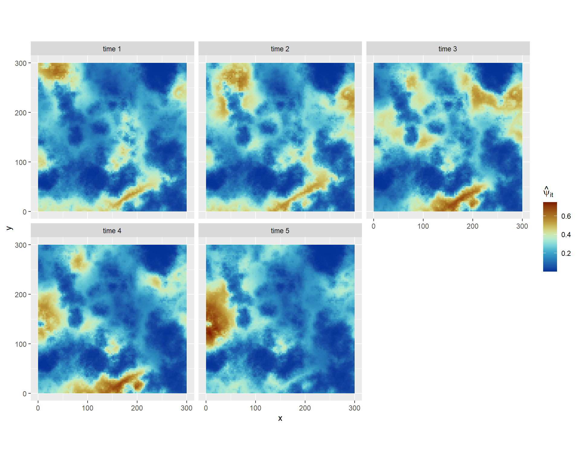
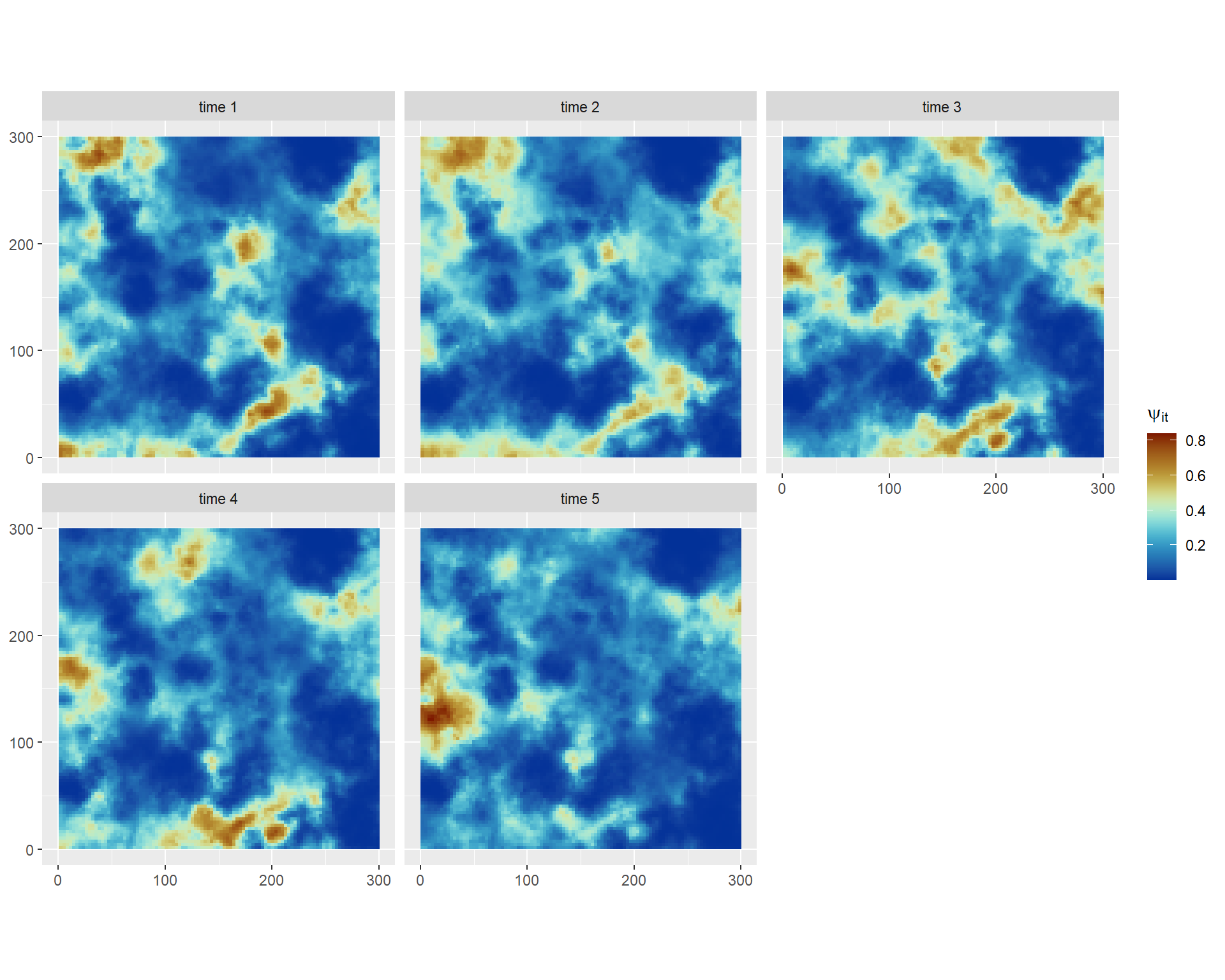
We can compare these results against the true simulated values downloadable here:
3 Space varying coefficients (SVC) model
3.1 Continuous space-varying trend
In this section we will fit the following SVC occupancy model:
\[\begin{align} z_{it} &\sim \mathrm{Bernoulli}(\psi_{it}) \nonumber \\ \mathrm{logit}(\psi_{it}) &= \beta_0 + \beta_{1}(i) t + \omega(i)\nonumber \\ y_{ijt} &\sim \mathrm{Bernoulli}(z_{it} \times p_{ijt})\nonumber\\ \mathrm{logit}(p_{ijt}) &= \alpha_0 + \alpha_1 \mbox{g}_{ijt}, \label{eq:occ_model3} \end{align}\]where the logit-scaled occupancy probabilities at locations \(i\) on time \(t\) are modeled with a continuous-space varying trend \(\beta_{1}(i)\) , a fixed intercept \(\beta_{0}\) (although a spatially varying intercept \(\beta_{0}(i)\) could be easily fitted as well), and \(\omega(i)\), a Gaussian random field with Matérn covariance function. The detection probabilities and observed occurrences are modeled in the same way as before.
| cellid | y1 | y2 | y3 | g1 | g2 | g3 | time | x.loc | y.loc | scale_time |
|---|---|---|---|---|---|---|---|---|---|---|
| 2 | NA | 1 | 1 | -0.66 | 0.00 | -0.35 | 1 | 4.5 | 1.5 | -1.41 |
| 2 | 0 | 0 | 0 | 0.09 | 0.87 | -0.94 | 2 | 4.5 | 1.5 | -0.71 |
| 2 | 0 | 0 | 0 | 0.26 | 0.63 | -0.13 | 3 | 4.5 | 1.5 | 0.00 |
| 2 | 0 | 0 | 0 | -0.10 | 0.93 | -0.70 | 4 | 4.5 | 1.5 | 0.71 |
| 2 | 1 | 1 | NA | 0.74 | -0.51 | 0.92 | 5 | 4.5 | 1.5 | 1.41 |
| 5 | 0 | 0 | 0 | -0.08 | 0.21 | 0.74 | 1 | 13.5 | 1.5 | -1.41 |
First, the SPDE model is defined by using PC-priors for the model parameters.
Code
boundary_sf = st_bbox(c(xmin = 0, xmax = 300, ymax = 0, ymin = 300)) %>%
  st_as_sfc() %>% st_as_sf()

mesh = fm_mesh_2d(loc.domain = st_coordinates(boundary_sf)[,1:2],
                    offset = c(-0.1, -.2),
                    max.edge = c(15, 30))

spde <- inla.spde2.pcmatern(mesh = mesh,
                              prior.range = c(100, 0.5),
                              prior.sigma = c(1, 0.5))
Now we prepare and fit the data
Two sets of indexes need to be created for (i) the spatial field and (ii) the spatio-temporal component.
iset_sp1 <- inla.spde.make.index(name = "i1",
                                 n.spde =  spde$n.spde)

iset_sp2 <- inla.spde.make.index(name = "i2",
                                 n.spde =  spde$n.spde)
For the Spatial field \(\omega(i)\), the projector matrix A mapping the model domain to the data locations is computed. As for the space-varying trend, this is represented as the Kronecker product of the projector matrix and the covariate vector, i.e., \((\mathbf{A}\otimes (\mathbf{x1})^T))\beta_1\) . Such computation is done internally within the inla.spde.make.A() function when the covariate vector gets passed on to the weights argument (in this case, the scaled-time covariate).
A_sp1 <- inla.spde.make.A(mesh = mesh,
                         loc = as.matrix(svc_data[,c("x.loc","y.loc")]))
#space-time projector matrix
A_sp2 <- inla.spde.make.A(mesh = mesh,
                          loc = as.matrix(svc_data[,c("x.loc","y.loc")]),
                          weights = svc_data$scale_time)
For building the stack both projector matrices and indexes must be specified.
Y_mat <- svc_data %>%
  dplyr::select(num_range("y",1:3)) %>%
  as.matrix()
X_det <- svc_data %>%
  dplyr::select(num_range("g",1:3)) %>%
  inla.Occupancy_detCov()
X_cov <- svc_data %>%
  dplyr::select(c(time,scale_time)) %>%
  mutate(Int_occ = 1)

stk <- inla.stack(data=list(Y= Y_mat, X = X_det),
                  A=list(A_sp1,A_sp2,1),
                  effects=list(iset_sp1,
                               iset_sp2,
                               as.list(X_cov)),

                  tag='SVC')
The model formulas include both spde models, which are then passed on to the inla function (note that we have used Empirical Bayes integration strategy for computational purpose, see Gómez-Rubio (2020) for further details).
Code
formula_svc = inla.mdata(Y,X) ~
  -1 + Int_occ +
  f(i1, model=spde)  +
  f(i2, model=spde)

model_svc <- inla(formula_svc, #the formula
              data=inla.stack.data(stk),
              family= 'occupancy',
              control.fixed =  list(prec = 1, prec.intercept = 1),
              control.predictor=list(A=inla.stack.A(stk),
                                     compute=TRUE),
              control.compute = list(dic = TRUE, waic = TRUE,
                                     config = TRUE),
              # verbose = TRUE,
              control.inla = list(int.strategy = "eb"),
              control.family = list(control.link = list(model = "logit"),
                                    link.simple = "logit",
                       hyper = list(beta1 = list(param = c(0,1/3),
                                                              initial = 0),
                                    beta2 = list(param = c(0,1/3)))
                       ))
Warning in normalizePath(path.expand(path), winslash, mustWork):
path[1]="C:/Users/jaf_i/AppData/Local/Temp/Rtmp4wvNAp/file128a82e2d6c7f": The
system cannot find the file specifiedFor the Spatial field \(\omega(i)\), the projector matrix A mapping the model domain to the data locations is computed. As for the space-varying trend, this is represented as the Kronecker product of the projector matrix and the covariate vector, i.e., \((\mathbf{A}\otimes (\mathbf{x1})^T))\beta_1\) . Such computation is done internally within the inla.spde.make.A() function when the covariate vector gets passed on to the weights argument (in this case, the scaled-time covariate).
A_sp1 <- inla.spde.make.A(mesh = mesh,
                         loc = as.matrix(svc_data[,c("x.loc","y.loc")]))

#space-time projector matrix

A_sp2 <- inla.spde.make.A(mesh = mesh,
                          loc = as.matrix(svc_data[,c("x.loc","y.loc")]),
                          weights = svc_data$scale_time)
We can create a list containing the detection/non-detection matrix, the detection covariates, and a list containing the the intercept column for the base-line occupancy, the time points, and two empty vectors (since both space and space-time A projector matrices are provided in the A.local argument).
Y_mat <- svc_data %>%
  dplyr::select(num_range("y",1:3)) %>%
  as.matrix()
X_det <- svc_data %>%
  dplyr::select(num_range("g",1:3)) %>%
  inla.Occupancy_detCov()
X_cov <- svc_data %>%
  dplyr::select(time,scale_time) %>%
  mutate(Int_occ = 1,
         i1 = NA,
         i2 = NA)

data_list <- as.list(X_cov)
data_list$X <- X_det
data_list$Y <- Y_mat
The model formula includes both spde models, which are then passed on to the inla function (note that we have used Empirical Bayes integration strategy for computational purpose, see Gómez-Rubio (2020) for further details).
formula_svc = inla.mdata(Y,X) ~
  -1 + Int_occ +
  f(i1, model=spde, A.local = A_sp1)  +
  f(i2, model=spde, A.local = A_sp2)

model_svc <- inla(formula_svc, #the formula
              data=data_list,
              family= 'occupancy',
              control.fixed =  list(prec = 1, prec.intercept = 1),
              control.compute = list(dic = TRUE, waic = TRUE,
                                     config = TRUE),
              # verbose = TRUE,
              control.inla = list(int.strategy = "eb"),
              control.family = list(control.link = list(model = "logit"),
                                    link.simple = "logit",
                                    hyper = list(beta1 = list(param = c(0,1/3),
                                                              initial = 0),
                                                 beta2 = list(param = c(0,1/3),
                                                              initial = 0))))
3.2 Visualize space-varying trend
To plot the predicted spatial trend, a fine grid covering the spatial domain must be created. We can use sf::st_make_grid() function to do this.
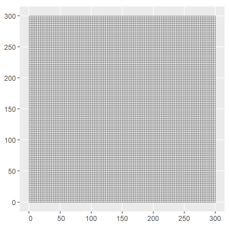
Once the prediction grid is created, a projector matrix A_pred is computed based on the locations of the grid. Posterior samples of the model are drawn, and the projector matrix is used to evaluate the spatio-temporal trend on the samples.
# projector matrix
A_pred = inla.spde.make.A(mesh, st_coordinates(projection_grid))

# samples
samples = inla.posterior.sample(1000, model_svc)

# evaluate the spatial temporal trend
svc_eval = inla.posterior.sample.eval(function(x) (A_pred %*% i2)[,1],

                                 samples)
We can compute the posterior mean, median, quantiles, and also check for significance. This information can be appended into a prediction data frame and converting it to a SpatRaster for visualization.
Code
dd = data.frame(x = st_coordinates(projection_grid)[,1],
                y = st_coordinates(projection_grid)[,2],
                z = apply(svc_eval,1,mean),
                q1 = apply(svc_eval,1,quantile,0.025),
                q2 = apply(svc_eval,1,quantile,0.975)) %>%
  mutate(check = case_when( q1>=0 & q2>=0 ~1,

                             q1<0 & q2<0 ~ -1,

                             q1<0 & q2>0 ~ 0)) %>%
  terra::rast()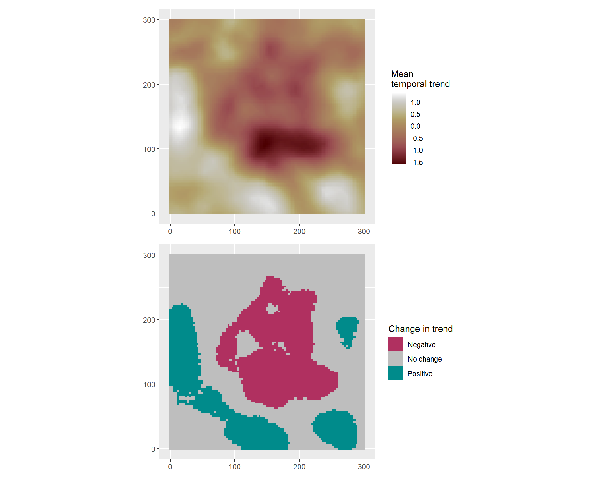
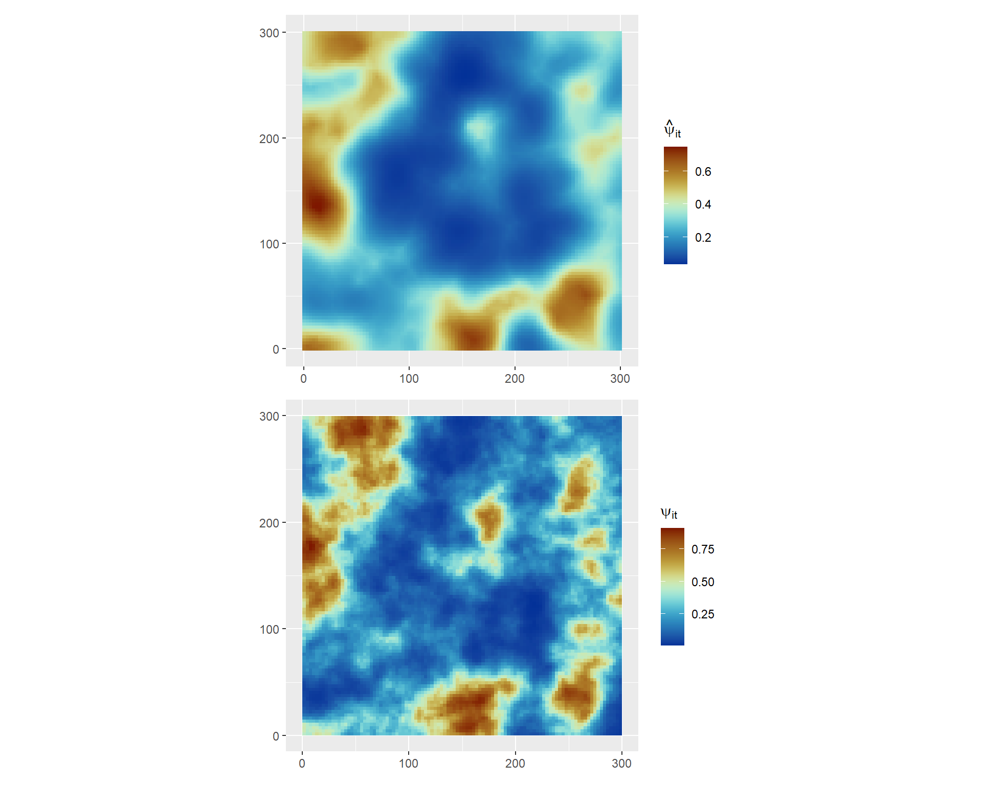
We can also compute a the predicted occupancy probabilities at a fixed time point \(t\) by evaluating the linear predictor on the posterior samples. We define a function func_svc() to compute the the liner predictor for a given time point.
For example, for \(t=5\) we can compute the posterior mean occupancy probability as follows:
Code
# select t= 5

time=5

# evaluate the linear predictor on the posterior samples

eta_post = inla.posterior.sample.eval(func_svc, samples, time = 5)

dd2 = data.frame(x = st_coordinates(projection_grid)[,1],
                y = st_coordinates(projection_grid)[,2],
                psi =apply(inla.link.logit(eta_post, inverse = T),1,mean)) %>%

  terra::rast()
Now we can compare this result against the true simulated values available to be downloaded:
3.3 Regional Varying Trend
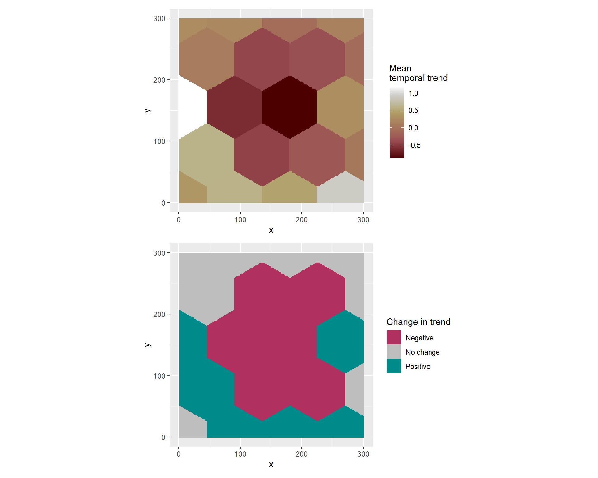
Now suppose we are interested in modelling the regional varying trend \(\beta_{R_i}\) for a set of \(p\) non-overlapping regions over the spatial domain, i.e. \(\mathcal{D} = \bigcup\limits_{i=1}^p R_i\) such that \(R_i\bigcap R_j = \emptyset\) for each \(i\neq j\). We can discretized the study area into 20 regions as follows:
Code
R_i <- st_make_grid(boundary_sf, cellsize = 90, square = FALSE) %>%
    st_cast("MULTIPOLYGON") %>%
  st_sf() %>%
  mutate(cellid = row_number()) %>%
  st_crop(boundary_sf) %>%
  st_collection_extract( "POLYGON") %>%
  mutate(cellid = 1:length(cellid))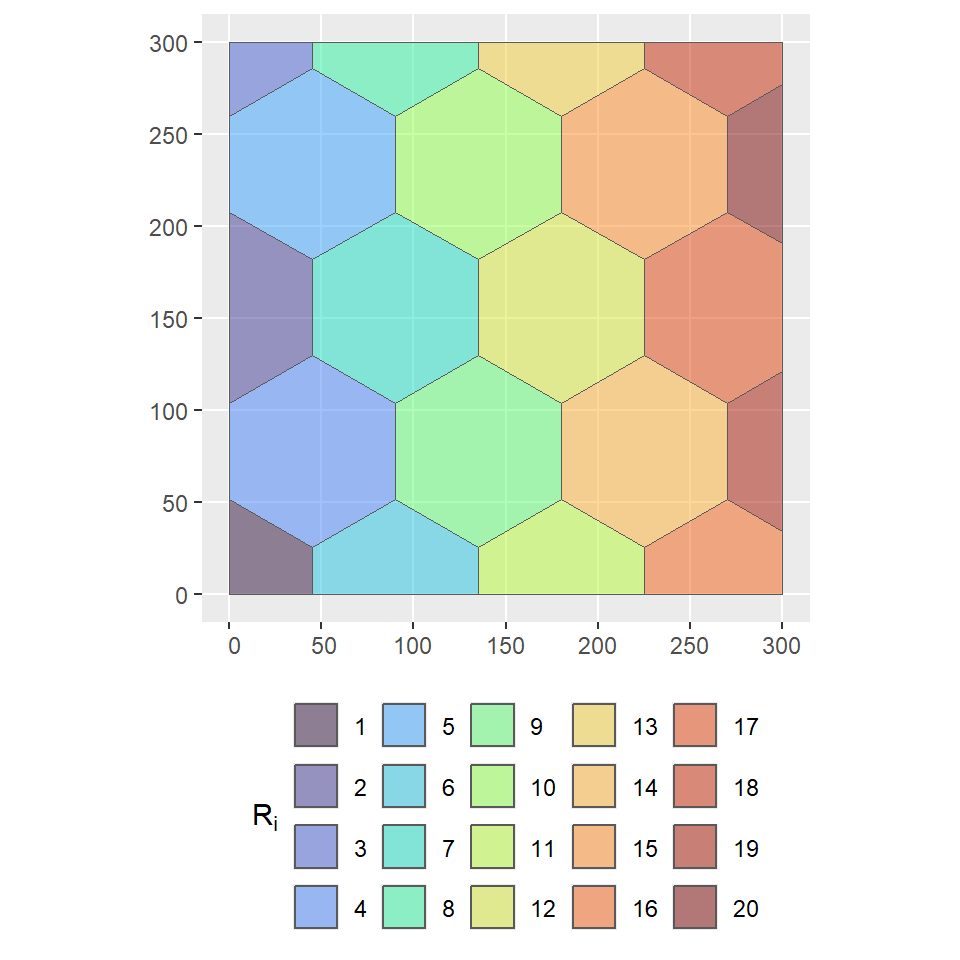
The regional varying trend \(\beta_{R_i}\) in the linear predictor can be vary across the \(p\) discrete aerial units through \(iid\) random effects, or according to a spatial dependence structure modeled with an areal spatial process. For the latter case, the spatial structure is usually described by neighborhood matrices. The R-package spdep facilitates building a neighbors list based on the defined regions and then generates a weights matrix \(\mathbf{W}\) (e.g. \(w_{ij} = 1\) if region \(i\) is neighbor of \(j\) and zero otherwise) .
Next, we find the region id where each observation lies and append this information to the data set.
The spatial relationships can be described by one of INLA’s available areal spatial models (see inla.list.models("latent") for a list of the latent models available in INLA). In this example, we will use the Besag-York-Mollié model (BYM) which is an extension to the intrinsic CAR model that contains an i.i.d. model component for the non-spatial heterogeneity, i.e.
Thus, slopes are sampled from a normal distribution, where the conditional mean is linked to the average of neighboring cells and a conditional variance proportional to the variance across adjacent cells and inversely proportional to the number of adjacent cells.
For fitting this model in INLA we need a spatial index for the spatial field \(\omega(i)\) and projection matrix to map the model domain to the coordinates of the data.
iset_sp <- inla.spde.make.index(name = "spatialfield",
                                n.spde =  spde$n.spde)

A_sp <- inla.spde.make.A(mesh = mesh,
                         loc = st_coordinates(svc_data_R))
We also need to supply the region index from the data as a numerical input in the stack effects list.
stk <- inla.stack(data=list(Y = Y_mat, X =X_det),
                  A=list(A_sp,1),
                  effects=list(iset_sp,
                               data.frame(Int_occ = 1,
                                    region_id = svc_data_R$cellid,
                                    scale_time = svc_data_R$scale_time,
                                    time = svc_data_R$time)),
                  tag='SVC_R')
To fit the regional varying trend model with BYM structured spatial effects, the component related to the space-varying coefficient in the model formula must contain:
The region id (as defined in the data stack)
The covariate value (in this case the scaled-time)
The CAR model (
model ="bym")The weight matrix \(\mathbf{W}\)
formula_svc_R = inla.mdata(Y,X) ~
  -1 + Int_occ +
  f(region_id,scale_time, model = "bym", graph = W.nb)  +
  f(spatialfield, model = spde)
We will save the inla output as model_svc_R :
Code
model_svc_R <- inla(formula_svc_R, #the formula
              data=inla.stack.data(stk),
              family= 'occupancy',
              control.fixed =  list(prec = 1, prec.intercept = 1),
              control.predictor=list(A=inla.stack.A(stk),
                                     compute=TRUE),
              control.compute = list(dic = TRUE, waic = TRUE,
                                     config = TRUE),
              control.inla = list(int.strategy = "eb"),
              control.family = list(control.link = list(model = "logit"),
                                    link.simple = "logit",
                                    hyper = list(beta1 = list(param = c(0,1/3),
                                                              initial = 0),
                                                 beta2 = list(param = c(0,1/3),
                                                              initial = 0))
                                    ))
Warning in normalizePath(path.expand(path), winslash, mustWork):
path[1]="C:/Users/jaf_i/AppData/Local/Temp/Rtmp4wvNAp/file128a8435a2d18": The
system cannot find the file specifiedFor fitting this model in INLA we create the projection matrix to map the model domain to the coordinates of the data.
A_sp <- inla.spde.make.A(mesh = mesh,
                         loc = st_coordinates(svc_data_R))
We create a list with the detection/non-detection data, detection covariates and a list of occupancy covariates including the time and region indeces/
To fit the regional varying trend model with BYM structured spatial effects, the component related to the space-varying coefficient in the model formula must contain:
formula_svc_R = inla.mdata(Y,X) ~
  -1 + Int_occ +
  f(region_id,scale_time, model = "bym", graph = W.nb)  +
  f(spatialfield, model = spde, A.local = A_sp)

model_svc_R <- inla(formula_svc_R, #the formula
              data=data_list,
              family= 'occupancy',
              control.fixed =  list(prec = 1, prec.intercept = 1),
              control.compute = list(dic = TRUE, waic = TRUE,
                                     config = TRUE),
              control.inla = list(int.strategy = "eb"),
              control.family = list(control.link = list(model = "logit"),
                                    link.simple = "logit",
                        hyper = list(beta1 = list(param = c(0,1/3),
                                                              initial = 0),
                                    beta2 = list(param = c(0,1/3),
                                                              initial = 0))
                        ))
To visualize the results we can take the prediction grid created for the prediction of the continuous-space varying trend model and index each cell according to the region \(R_i~\mbox{for } i = 1,\ldots,20\).
# add cellid to prediction grid

projection_grid_R <- st_intersection(projection_grid,R_i)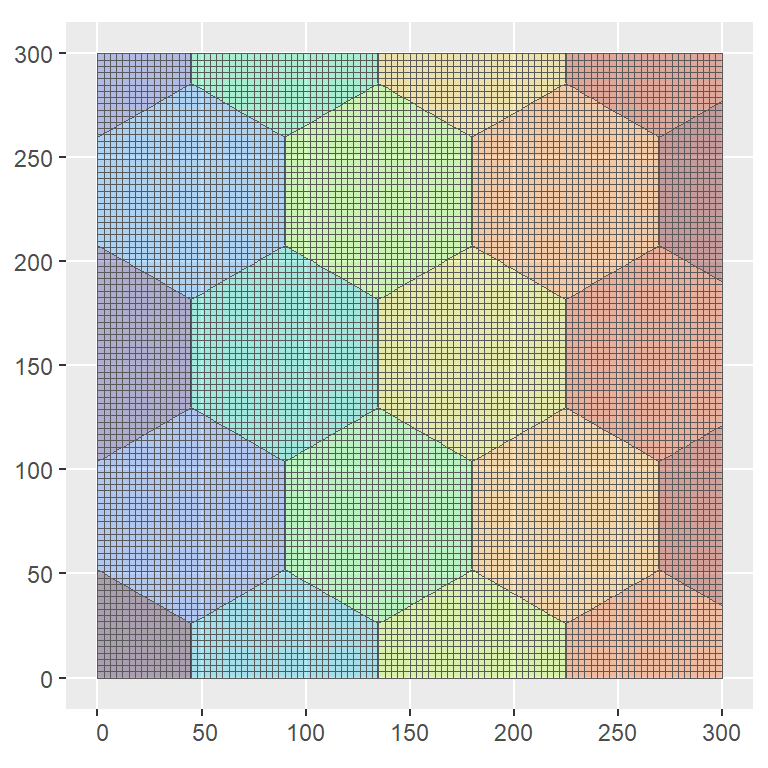
Next, we compute posterior samples of the model to evaluate the trend for each cell indexed by region \(R_i\).
# samples
samples = inla.posterior.sample(1000, model_svc_R)
# evaluate the spatial temporal trend

svc_eval_R = inla.posterior.sample.eval(function(x)
  (region_id[projection_grid_R$cellid]), samples)
Finally, we can compute posterior quantities (i.e. the mean, quantiles, etc) and check for significance. This information can be appended directly into the prediction grid which can be then be rasterized using the stars R-package for visualization purposes.
# append to prediction grid

projection_grid_R =projection_grid_R %>%
  mutate( z = apply(svc_eval_R,1,mean),
          q1 = apply(svc_eval_R,1,quantile,0.025),
          q2 = apply(svc_eval_R,1,quantile,0.975),
          check = case_when( q1>=0 & q2>=0 ~1,

                             q1<0 & q2<0 ~ -1,

                             q1<0 & q2>0 ~ 0))

# Rasterize
regional_trend <-stars::st_rasterize(projection_grid_R)