Point process modelling inlabru

The general idea is to fit a LGCP that includes (1) a spatial covariate (elevation in this case) and (2) an SPDE to account for unexplained spatial variation. Spatial covariates can be available in different formats. In the gorillas example, the elevation variable is available as SpatialPixelsDataFrame spatial-class object but we will convert it to a raster as this is in many data sets spatial covariates are read as raster data.

Note

Note that inlabru articles on the website have already been updated and thus, the material in here is very similar to the one found online. We will use the gorillas_sf data which contains an updated version of the variables in the original data set.

Firs we will begin reading the data:

library(INLA)
library(sf)
library(inlabru)
library(stars)
library(terra)
library(ggplot2)
library(tidyterra)
# Data sets 

data(gorillas_sf)

nests <- gorillas_sf$nests
mesh <- gorillas_sf$mesh
boundary <- gorillas_sf$boundary
gcov <- gorillas_sf_gcov()

ggplot() +
  gg(mesh) +
  geom_sf(data = boundary, alpha = 0.1, fill = "blue") +
  geom_sf(data = nests) +
  ggtitle("Points")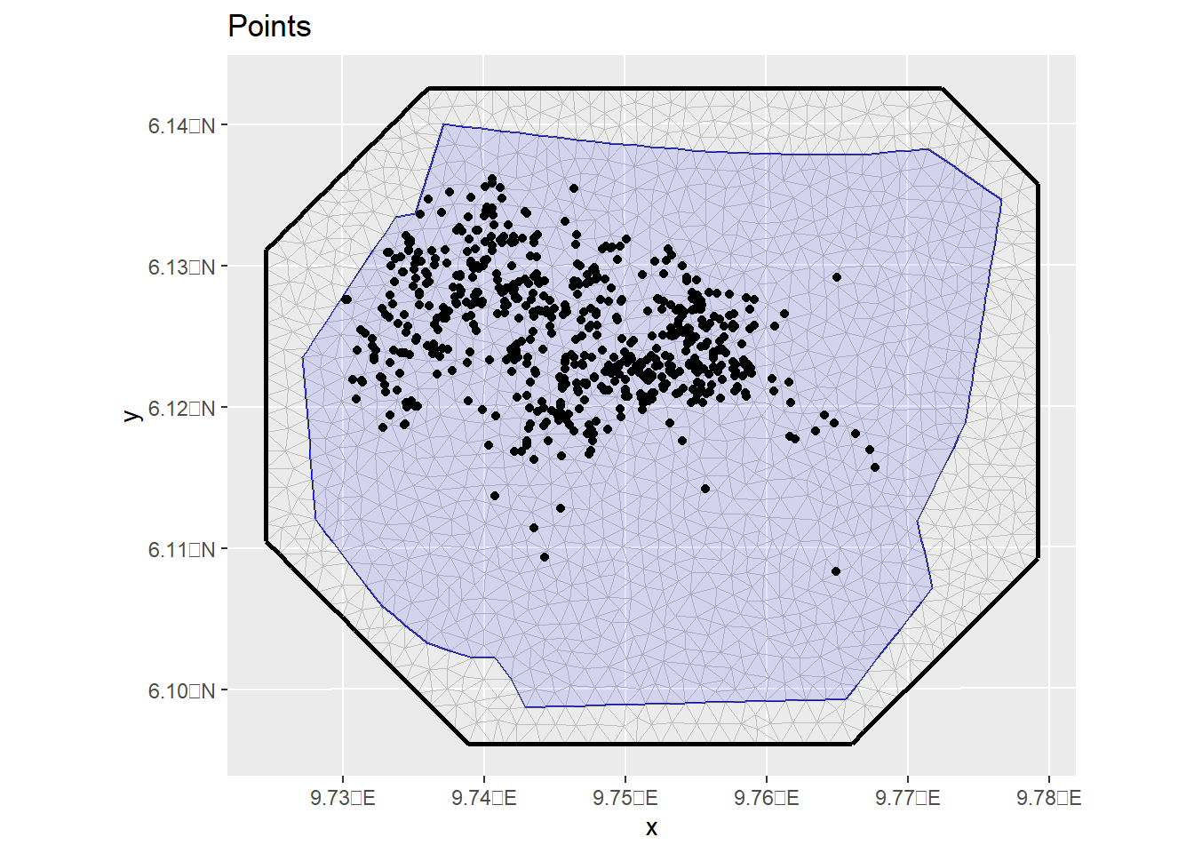

Now we define the model components. Recall for a LGCP (and point process in general) we need the covariates to be available everywhere. Thus, we can specify the following:

eval_spatial(raster, where=geometry,...)

raster covariates can be of any class supported by eval_spatial. Note that eval_spatial would be called automatically for raster inputs:

comp3a <- geometry ~ elevation(gcov$elevation, model = "linear")
fit3a <- lgcp(comp3a, nests, samplers = boundary, domain = list(geometry = mesh))
fit3a$summary.fixed

However, if it doesn’t auto detect it then you should call the eval_spatial:

comp3b <- geometry ~ elevation(eval_spatial(data=gcov$elevation,where = .data.), model = "linear")
fit3b <- lgcp(comp3b, nests, samplers = boundary, domain = list(geometry = mesh))
fit3b$summary.fixed

                  mean           sd   0.025quant     0.5quant   0.975quant
elevation  0.004194011 0.0002466676  0.003710552  0.004194011  0.004677471
Intercept -3.817061673 0.4464031906 -4.691995849 -3.817061673 -2.942127497
                  mode kld
elevation  0.004194011   0
Intercept -3.817061673   0

Here, where = .data. is bascially telling where do we want to evaluate. In this case we look for the geometry column in the data input . so the same results could be obtained by calling directly the name of the column as:

 geometry ~ elevation(eval_spatial(data=gcov$elevation,where = geometry), model = "linear")

Since we want to evaluate the covariate at arbitrary points in the survey region we want these values to be defined everywhere. So if the values of a raster are missing for certain evaluation points, inlabru will impute it with the nearest-available value.

elevation_missing <- gcov$elevation
values(elevation_missing)[values(elevation_missing)==2008] <- NA
ggplot()+geom_spatraster(data = elevation_missing)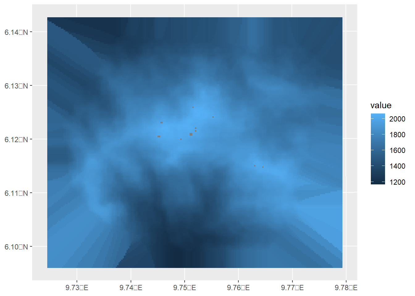

comp3_missing <- geometry ~ elevation(elevation_missing, model = "linear")
fit3_miss <- lgcp(comp3_missing, nests, samplers = boundary, domain = list(geometry = mesh))

Warning in input_eval.bru_input(subcomp$input, data = lh$data, env = env, : Model input 'elevation_missing' for 'elevation' returned some NA values.
Attempting to fill in spatially by nearest available value.
To avoid this basic covariate imputation, supply complete data.

Warning in input_eval.bru_input(component[[part]]$input, data, env = component$env, : Model input 'elevation_missing' for 'elevation' returned some NA values.
Attempting to fill in spatially by nearest available value.
To avoid this basic covariate imputation, supply complete data.

fit3_miss$summary.fixed

                  mean           sd   0.025quant     0.5quant   0.975quant
elevation  0.004193971 0.0002466463  0.003710553  0.004193971  0.004677389
Intercept -3.816986410 0.4463657581 -4.691847220 -3.816986410 -2.942125601
                  mode kld
elevation  0.004193971   0
Intercept -3.816986410   0

Alternatively, we could write a function that does this for us (we use bru_fill_missing to impute the missing values) :

f.elev <- function(raster,where) {
  # Extract the values
  v <- eval_spatial(raster, where)
  # Fill in missing values
  if (any(is.na(v))) {
    v <- bru_fill_missing(raster, where, v)
  }
  return(v)
}

comp3_in <- geometry ~ elevation(f.elev(raster = elevation_missing,where = .data.), model = "linear")
fit3_in <- lgcp(comp3_in, nests, samplers = boundary, domain = list(geometry = mesh))
fit3_in$summary.fixed

                  mean           sd   0.025quant     0.5quant   0.975quant
elevation  0.004193971 0.0002466463  0.003710553  0.004193971  0.004677389
Intercept -3.816986410 0.4463657581 -4.691847220 -3.816986410 -2.942125601
                  mode kld
elevation  0.004193971   0
Intercept -3.816986410   0

Lets fit now a LGCP including a continuous spatial effects and an elevation effect.

matern <- inla.spde2.pcmatern(
  mesh,
  prior.sigma = c(0.1, 0.01),
  prior.range = c(0.05, 0.01)
)

comp_lgcp <- geometry ~ Intercept(1)  +
             elevation(gcov$elevation, model = "linear")+
             field(geometry, model = matern)

fit_lgcp <- lgcp(comp_lgcp, nests, 
                 samplers = boundary, 
                 domain = list(geometry = mesh))

Important

Notice that for a model with an intercept only we need to tell the correct size :

 geometry ~ 0 + Intercept(rep(1, nrow(.data.)), model = "linear")

Now we can estimate the abundance by computed the integrated intensity \(\lambda_{int}\) over the domain. To do so, we first obtain the integration points using the fm_int function which contains the integration weight values:

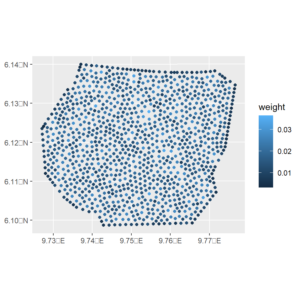
Lambda <- predict(
  fit_lgcp,
  fm_int(mesh, boundary),
  ~ sum(weight * exp(Intercept + elevation + field))
)
Lambda

      mean       sd   q0.025     q0.5   q0.975   median mean.mc_std_err
1 682.7261 26.77353 638.6272 681.0564 743.4143 681.0564        2.677353
  sd.mc_std_err
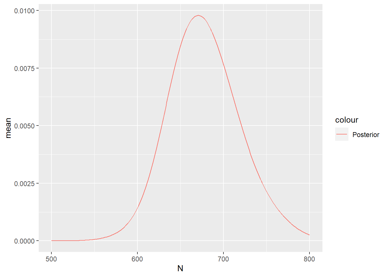
1      2.072871

Given this values of \(\lambda_{int}\) we can estimate the posterior abundance as follows:

Nest <- predict(
  fit_lgcp,
  fm_int(mesh, boundary),
  ~ data.frame(
    N = 500:800,
    dpois(500:800,
      lambda = sum(weight * exp(Intercept + elevation + field))
    )
  )
)

ggplot(data = Nest) +
  geom_line(aes(x = N, y = mean, colour = "Posterior"))